Multioutput Gaussian Processes for Loss Ratio Development

1. Introduction

Property and casualty insurance claims often have a long tail, meaning they can take years, or even decades, to fully materialize and realize their full cost. As a result, insurers are responsible for estimating a reasonable loss reserve to cover future unknown costs that may arise from these claims. The adequacy of these loss reserves is a significant financial risk for insurers, as excessive or inadequate reserves can lead to financial strain. In recent years, the discussion on loss reserves has evolved from using reasonable point estimates to also considering reliable distributions of uncertainty. Such distributions can provide a more comprehensive assessment of the risk associated with loss reserves, helping insurers to more accurately gauge the potential financial impact of their reserve estimates.

Stochastic models are a valuable tool for estimating the distribution of loss reserves, as they can help actuaries capture the uncertainty inherent in the claims process. Early attempts included variations of the chain ladder method (Mack 1993, 1994), but such models were limited in their ability to provide adequate measures of uncertainty (Meyers 2015). To assist researchers in comparing new models, Meyers developed a retrospective testing framework to evaluate the reserves in terms of both point and distributional accuracy. Among the many different models that have been developed for estimating loss reserves, Bayesian methods have emerged as a popular choice due to their ability to incorporate prior knowledge, model hierarchical relationships and complex distributions, quantify uncertainty, and handle missing data.

We will focus on one subset of Bayesian models: Gaussian processes (GPs). GPs are a highly flexible modeling technique, and they are widely used for analyzing time series data. One of the key strengths of GPs is their ability to capture the correlation between different time periods, making them well suited for modeling loss development patterns. GPs also have the advantage of being able to estimate multiple sources of uncertainty, which is important when dealing with complex and uncertain data. In this paper, we also leverage the highly customizable formulation of GPs to incorporate known structural information about loss ratio triangles and cross-triangle relationships into our model.

1.1. Computational tractability

Throughout this paper, we refer to models sampled using Markov chain Monte Carlo (MCMC) methods. MCMC methods are popular because they can sample from a wide range of distributions, including complex distributions that may not have an analytical form. In addition, these methods have the property of convergence, which means that as the training set grows, the sample mean and variance of the distribution converge toward the true mean and variance. This makes them a reliable tool for approximating the posterior distribution of model parameters given some observed data. That said, they can be slow and may not scale well with large datasets.

Computational tractability is an especially important issue in the use of GP models, as the computational complexity of exact GP inference grows cubically with the number of data points (Rasmussen and Williams 2006). This can make it challenging to scale GP models to large datasets. In this paper, a single-output GP model for one company, line, and loss type combination usually completes in about two minutes, while a comparable multioutput model takes about eight minutes with training sets of 55 and 110 data points, respectively. In practice, larger triangles or more triangle types could be modeled using the method presented in this paper, and it may be beneficial to adjust the data or simulation method.

One alternative to MCMC for GP inference is the use of variational approximations, which seek to find a tractable distribution that is close to the true posterior. Such methods can be faster than MCMC and are often easier to scale to large datasets, but they may not be as accurate. While there are efforts to create model-agnostic formulations of variational inference (Kucukelbir et al. 2015), the current best practice is to develop model-specific calculations, which is beyond the scope of this paper.

Another possibility is to use subset selection methods, which select a small subset of the data to use in GP inference and approximate the rest of the data using a cheaper method. This can be effective if the data exhibits some form of structure or regularity that allows for accurate approximations. This is clearly applicable to loss ratio development because loss ratios in later development periods stabilize greatly. While early periods may be best modeled in development quarters, gaps in later periods may extend multiple years. Reducing the dataset in this way could sufficiently inform the GP while limiting the time spent sampling.

1.2. Gaussian processes for loss development

In recent years, GP modeling has been applied to the analysis of loss development patterns in insurance. Two notable examples are the studies by Lally and Hartman (2018) and Ludkovski and Zail (2021). Both approaches involve representing the loss development triangle as a two-dimensional surface and modeling the relationships between points within the triangle.

The use of GP models for loss development analysis has several benefits. These include the ability to extrapolate losses into tail periods with a tunable structure, quantify uncertainty over multiple experience periods, capture calendar year trends, and apply a type of actuarial credibility from data underlying the historical loss development patterns.

Lally and Hartman (2018) focus on modeling cumulative paid losses, which tend to exhibit smooth, monotonically increasing patterns. In their approach, they use input warping to restructure the triangle and effectively change the parameterization of the GP over time and space. This is particularly useful for capturing the rapid changes that often occur in the early stages of loss development, which tend to stabilize in later periods.

Ludkovski and Zail (2021) choose to model incremental paid loss ratios instead to adhere to an assumption of spatial dependence more closely. They employ a compound covariance function that shifts to linear extrapolations in areas with limited data and use a hurdle likelihood and virtual observations to overcome undesired predictions and inform the development shape. The noise in their model is also made to vary with the development lag, with the assumption that it will progressively decay over time.

1.3. Incorporating anisotropy

In a standard GP model, the relationship between points is defined purely by their distance in input space. This property, being invariant to rotations of the input space, is referred to as isotropy. Both GP models discussed above allow their parameterization to differ along the experience and development period dimensions. This is referred to as anisotropy. This is important to differentiate the impact of the trends within an experience period and those across experience periods.

However, the use of the trend across experience periods may effectively disappear when increasing the number of observations if the related parameters do not also vary with development lag. See Appendix A for an example using the Lally and Hartman (LH; 2018) model.

In cumulative loss or loss ratio models, it is essential to consider the relative increase in predictive power as the development lag increases for experience period–specific patterns. During early development periods, the information shared across experience periods is generally more informative and relevant than the early loss emergence of a new experience period. As the experience period develops and we gain more knowledge about the specific payout behavior of its claims, the relative importance of information shared across experience periods will decrease. Additionally, the cumulative losses across experience periods at similar points in development tend to diverge over time, which naturally reduces the usefulness of correlation across periods. As the experience period develops, the year-specific pattern correlation tends to approach 1, indicating that the patterns within the same experience period become more informative than patterns across different experience periods.

In incremental loss ratio models, the cross-period relationships are still more important in early development periods. The change in importance throughout the rest of development is less clear but should be informed by the data. This, like cumulative models, suggests a more flexible incorporation of anisotropy.

1.4. Paid and incurred projections

The dependency between paid and incurred loss triangles has long been an interest of practicing actuaries and researchers. The Munich chain ladder (Quarg and Mack 2008) extends the Mack chain ladder method to incorporate correlations between the paid and incurred development triangles. Making use of a paid-to-incurred ratio triangle and its reciprocal, the method incorporates deviances from the average payout pattern to inform the development factors of both paid and incurred losses. Importantly, the authors note, “the paid and incurred development factors contribute to the concurrence of paid and incurred” (Quarg and Mack 2008, 279). In the context of our GP models, it is likely that improvements in the accuracy of both paid and incurred loss projections can be achieved by correctly incorporating the dependency between these two types of losses.

The paid–incurred chain method (Happ and Wüthrich 2013) was developed to similarly incorporate correlation between paid and incurred loss triangles while allowing for accident year variation. Rather than two separate projections informed by one another, this method forces the ultimate paid and incurred claims to converge at the chosen ultimate development period. A correlation matrix is developed to model the dependence between loss patterns, assuming a multivariate Gaussian.

Like these models, a GP can adapt its loss type–specific projections to better adhere to known dependencies between loss types. The model structure we explore captures correlation between the paid and case incremental loss ratios across development lags, which we expect to increase over time. Here, case refers to the case reserves—estimates of future payments set by claims adjusters for reported but not fully settled claims. Incurred losses represent the total estimated liability and are defined as the sum of paid losses and case reserves. We will compare the performance of a single-output GP (SOGP) model with that of the multioutput GP (MOGP) model to assess relative performance.

1.5. Contribution

Our proposed MOGP uses shared learning to incorporate known dependencies between loss triangles and provides more flexibility in incorporating trends throughout the triangle. The model offers a general solution for any set of dependent triangles, but for demonstration purposes, we will examine results for paid and incurred losses. These cumulative losses are predicted by modeling incremental paid and case loss ratio triangles. Further segmentation of the losses into claim types, coverages, jurisdictions, and more can be explored with different datasets.

Actuaries are accustomed to reviewing separate development methods on a selected set of homogenous loss groups, like paid and incurred losses. A combination of multiple methods is generally accepted as a reasonable point estimate. Diagnostics to detect changes in the operational or external environment are used to weigh the reliability of different methods or otherwise adjust the final reserves. The primary benefit of the MOGP is to provide credible adjustments to loss projections using signal from other loss types with relationships derived from the data.

The presented MOGP implicitly adjusts for common environmental changes such as those in case reserve adequacy and settlement rate. Given the relationship between incremental paid and case loss ratio patterns and development time, the ultimate projections shift toward one another. For example, if case reserve adjustments are delayed in a particular experience period, the paid loss ratio pattern will likely adjust the incurred projections upward.

Shared learning also benefits noisy triangles. Whereas any set of triangles may be individually noisy, the available signal in each triangle informs the others, effectively reducing uncertainty throughout. For example, if an unusually large claim is reported early with a low payout, the model is less likely to overstate the incurred projection due to convergence toward the paid values over time. Similarly, it will also be less likely to understate paid losses. These benefits apply to areas of the triangle with limited data as well. Late development periods will have only a few data points in our training set, so incorporating multiple triangles will provide more confidence to the direction.

Relative to Ludkovski and Zail (2021), the MOGP avoids the use of hurdle likelihoods, allowing for triangle estimates with negative development. This includes some paid development patterns, all case reserve patterns, and most incurred patterns. Also, the MOGP uses the sum of one-dimensional nonstationary kernels to capture changes in trends and the relative importance of the year-specific and cross-year patterns. This more flexible structure better represents the data and dramatically decreases sampling time.

Finally, like Meyers (2015) and Ludkovski and Zail (2021), we thoroughly test our method on suitable paid and incurred loss triangles in the National Association of Insurance Commissioners (NAIC) dataset (Meyers and Shi 2021) described in the next section. We summarize ultimate loss point accuracy by loss type, line of business, and firm size. Distributional fits across loss types and lines of business are also compared. For each of these, we compare to a set of readily available methods, including the Mack chain ladder, the GP model from Lally and Hartman (2018), and the GP model with hurdle likelihoods and virtual observations from Ludkovski and Zail (2021). We exclude the Munich chain ladder throughout because too many results were deemed unreliable by the ChainLadder package available in R (Gesmann et al. 2025).

In alignment with the related work discussed above, we use the Stan language with RStan to implement the MOGP. This Bayesian modeling software uses Hamiltonian Monte Carlo sampling, which is state of the art for probabilistic inference. All models are run with default settings.

1.6. Data

We use the NAIC dataset (Meyers and Shi 2021) for development and testing purposes. The dataset comprises Schedule P triangles from 200 companies across six lines of business. The accident years range from 1988 to 1997 with net loss and premium data complete through the calendar year 1997.

The use of the NAIC dataset is consistent among authors with related topics committed to consistent and robust performance testing. In this paper, we only make use of companies with 10 complete years of data. The earned premium (EP) and loss values must also be positive for all years and development periods. Table 1 provides basic descriptions of our selected triangles.

The MOGP trains on a pair of upper-left triangles, each with 55 observations, and predicts the related 45 observations of each bottom-right triangle. All testing relies on cumulative loss at development lag 10—the last period available.

2. Gaussian process regression

A GP is the infinite-dimension generalization of a multivariate normal distribution. For any finite set of data X, a GP produces a random vector f(x) as a multivariate Gaussian random vector. Its infinite expansion of parameters translates to a nonparametric regression that can estimate any continuous function.

To efficiently learn the relationships between all points in time, the covariance matrix is parameterized with a kernel function. This reduces the total number of model parameters and provides an informed structure to the GP. The choice of kernel function is based on the known properties of the data. The most popular kernels relate covariance values to the distances between pairs of inputs. Thus, we can extend the GP prediction to any point at which we can calculate a distance. This is important for loss reserve estimation.

GP regression is defined like any regression with an input vector x within a continuous domain:

$$\begin{array}{c}y = f(x) + \varepsilon,\\ \varepsilon\sim\ N\left( 0,\sigma^{2} \right),\ \sigma^{2} \in \mathbb{R}^{+}.\end{array}\tag{2.1}$$

The inputs for a development triangle are two-dimensional: experience period and development lag. A Gaussian prior applies to the function f. We assume a zero mean, which is common. In other words, the function relies entirely on the parameterized covariance. The model of the function value is

$$f(x)\sim N\left( 0,\ k\left( x,\ x^{\mathstrut'} \right) \right). \tag{2.2}$$

This emphasizes the importance of choosing the correct kernel.

2.1. Kernel selection

The squared exponential (SE) kernel is one of the most widely used kernels in GP modeling. This kernel uses the distance between inputs to estimate the covariance and is characterized by two parameters: the lengthscale l and signal variance $\eta^{2}$. The lengthscale determines the smoothness of the function. A small lengthscale corresponds to a function with rapidly changing values, while a large lengthscale corresponds to a function with more gradual changes. Large lengthscales also allow for more reliable extrapolations. The signal variance, on the other hand, scales the variability of the function around the mean:

$$k_{SE}\left( x,\ x^{\mathstrut'} \right) = \eta^{2}e^{- \frac{\left( x - x^{\mathstrut'} \right)^{2}}{2l^{2}}}. \tag{2.3}$$

Since the covariance between two points relies solely on their relative distance, this kernel is stationary. This is inadequate for modeling loss ratio development, because

1. loss ratios change rapidly at the beginning of the development pattern, then stabilize over time, and

2. the variance of incremental loss ratios decreases over time.

This suggests we need a nonstationary kernel to accurately model our data. A nonstationary, generalized form of the SE kernel (Gibbs 1997) can be defined as

$$\small{k_{NSE}\left( x,\ x^{\mathstrut'} \right) = \eta(x)\eta\left( x^{\mathstrut'} \right)\sqrt{\frac{2l(x)l\left( x^{\mathstrut'} \right)}{{l(x)}^{2} + {l\left( x^{\mathstrut'} \right)}^{2}}}e^{- \frac{\left( x - x^{\mathstrut'} \right)^{2}}{{l(x)}^{2} + {l\left( x^{\mathstrut'} \right)}^{2}}}.} \tag{2.4}$$

In this kernel, the signal variance and lengthscales are dependent on x. Exactly how each parameter relates to development lag can be guided in the prior structure. One idea is to use GP priors on each kernel parameter (Heinonen et al. 2016), including an additional nonstationary noise term. This provides full flexibility but is likely to overcomplicate our problem and weaken extrapolation. Instead, we can rely on simplifying assumptions to constrain the distributions. For example, the lengthscale can remain constant after a selected development period.

2.3. Compound kernel

Compound kernels are a type of kernel used in GP modeling to capture complex relationships in the data that cannot be modeled by a single kernel function. They are formed, most commonly, by combining multiple valid kernels using either an additive or multiplicative approach (Rasmussen and Williams 2006, 95). In the additive approach, the compound kernel is formed by summing the individual kernel functions, each representing a different aspect of the data. An additive kernel model will suggest a strong relationship between time periods if any of the kernels suggest one. Alternatively, the multiplicative approach involves multiplying the individual kernel functions elementwise. A multiplicative kernel model will suggest a strong relationship only where all kernels agree.

For incremental development models, an additive approach makes more sense, while a multiplicative approach may be more suitable for cumulative loss models. This is due to the varying levels of spatial dependency. The incremental model benefits from layering relationships from the two dimensions throughout the triangle—hence, an additive kernel. The cumulative model has greater concern for removing correlation across experience periods as the development lag increases. Multiplying kernel values more easily allows for this.

In Section 1.3, we emphasized the importance of employing a nonstationary parameterization for the experience period dimension. Specifically, the impact of experience period should be allowed to vary with development lag, as it has a particularly strong influence in the early development periods. By adopting this approach, as the dataset informing the model expands and larger development lags become predominant in the sample, the model will continue to capture the underlying trends observed in the initial stages.

To accomplish this, we separate each dimension into its own kernel. The development and experience period dimensions will each use the nonstationary squared exponential as defined in equation (2.4). Both kernels will have their signal variance and lengthscales vary with the development period dimension. The resultant additive compound kernel is

$$\scriptsize{\begin{aligned} k_{C}(x,\ x') &= {\eta}_{1}\left( x_{1} \right){\eta}_{1}\left( x_{1}^{\mathstrut'} \right)\sqrt{\frac{2l_{1}\left( x_{1} \right)l_{1}\left( x_{1}^{\mathstrut'} \right)}{{l_{1}\left( x_{1} \right)}^{2} + {l_{1}\left( x_{1}^{\mathstrut'} \right)}^{2}}}e^{\frac{- \left( x_{1} - x_{1}^{\mathstrut'} \right)^{2}}{{l_{1}\left( x_{1} \right)}^{2} + {l_{1}\left( x_{1}^{\mathstrut'} \right)}^{2}}}\\ & \quad + {\eta}_{2}\left( x_{1} \right){\eta}_{2}\left( x_{1}^{\mathstrut'} \right)\sqrt{\frac{2l_{2}\left( x_{1} \right)l_{2}\left( x_{1}^{\mathstrut'} \right)}{{l_{2}\left( x_{1} \right)}^{2} + {l_{2}\left( x_{1}^{\mathstrut'} \right)}^{2}}}e^{\frac{- \left( x_{2} - x_{2}^{\mathstrut'} \right)^{2}}{{l_{2}\left( x_{1} \right)}^{2} + {l_{2}\left( x_{1}^{\mathstrut'} \right)}^{2}}}. \end{aligned}}\tag{2.5}$$

The x coordinate is defined as $\left( x_{1},x_{2} \right)$, where $x_{1}$ is the development period and $x_{2}$ is the experience period.

2.3. Linear model of coregionalization

To this point, the GP regression has a single output. In an MOGP, the covariance matrix must include the cross-covariance terms between outputs throughout the combined input space. The linear model of coregionalization (LMC) (Journel and Huijbregts 1978) achieves this with a linear combination of covariance matrices formed from the selected kernel. The number of matrices Q relates to the amount of flexibility needed to accurately model the data. A Q-length set of weight matrices is used to produce a linear combination of kernels. Given similar inputs for each output, the method simplifies to

$$k_{MO}\left( x,x^{\mathstrut'} \right) = \sum_{q = 1}^{Q}{B^{q} \otimes k^{q}(x,x^{\mathstrut'})}. \tag{2.6}$$

The $\otimes$ symbol represents the Kronecker product. For example, an LMC with Q = 2 and two outputs form the kernel

$$k\left( x,x^{\mathstrut'} \right) = \sum_{q = 1}^{2}{\left( \binom{b_{q,(1,1)}k^{q}(x,x^{\mathstrut'})}{b_{q,(2,1)}k^{q}(x,x^{\mathstrut'})}\binom{b_{q,(1,2)}k^{q}(x,x^{\mathstrut'})}{b_{q,(2,2)}k^{q}(x,x^{\mathstrut'})} \right),}$$

where the weight matrix is a symmetric positive definite matrix:

$$B^{q} = \left( \binom{b_{q,(1,1)}}{b_{q,(2,1)}}\binom{b_{q,(1,2)}}{b_{q,(2,2)}} \right).$$

This method can efficiently model a large set of outputs using sparsity-inducing priors to regularize the weight matrix (Cheng et al. 2020). However, in Cheng et al.'s model, they use a unique implementation to achieve convergence and reasonable run times. To sample effectively with standard settings in Stan, we use a different prior structure for the weight matrix (details in Section 3).

2.4. Incorporating noise

In addition to the kernels described in the prior sections, a nonstationary noise variance will be added at the triangle level in our model. This is an important distinction for the multioutput kernel (discussed in Section 2.3). Specifically, this means the noise variance is not included in the kernels but is instead added to their weighted product. This is not a meaningful distinction for the SOGP, which relies on one compound kernel.

A diagonal matrix $\Sigma$ will be added to the chosen kernel. For a multioutput model with T triangles, the noise matrix is

$$\Sigma = \begin{bmatrix} \Sigma_{1} & 0 & \cdots & 0 \\ 0 & \Sigma_{2} & \cdots & 0 \\ \vdots & \vdots & \ddots & \vdots \\ 0 & 0 & \cdots & \Sigma_{T} \end{bmatrix},$$

$$\Sigma_{t} = diag\left( \sigma_{t}^{2}\left( X_{1} \right) \right)\ for\ t \in \left\{ 1,2,\ldots,T \right\}. \tag{2.7}$$

Notice the noise parameter will only vary with $X_{1}$, i.e., there is a separate parameter for each development period d to account for the decreasing variance of incremental loss ratios within an experience period. Incorporating a noise adjustment by experience period may be useful but is not explored here.

2.5. Extrapolation

GP predictions are conditional on all observations y and reliant on the selected kernel. Derivations of the posterior for any set of hyperparameters or kernels use Bayes’ rule. Single and multioutput variations follow the same inferential formulation, predicting the set of outputs y* for a set of input vectors X*:

$$\scriptsize{\begin{array}{c} y^{*}\ \sim\ N\left( m^{*},\ \Sigma^{*} \right),\\ m^{*} = K(X^{*},X)({K(X,X) + \Sigma)}^{- 1}y,\\ \Sigma^{*} = K\left( X^{*},X^{*} \right) - K(X^{*},X)({K(X,X) + \Sigma)}^{- 1}{K\left( X^{*},X \right)}^{T}.\end{array}}\tag{2.8}$$

The stability of the kernel as x* moves further away from the trained observations affects the reliability of extrapolation. If the kernel parameters expand toward the range of their priors when predicting far into the future, the prediction is not likely useful.

3. Application to loss ratio development

Incremental paid and case loss ratio development patterns have a strong relationship and converge over time. Each can also be individually noisy. Combining the projection of these patterns allows for an increase in data without increasing the number of input variables (development and experience periods). For these reasons, an MOGP is uniquely suited to improve predictions and distributions of uncertainty. To support this conclusion, we also develop an SOGP on incremental paid and incurred loss ratios modeled separately with a similar prior structure.

3.1. Target variable

We choose to model the incremental paid and case loss ratios for a few reasons. First, incremental loss ratios maintain spatial dependence. This allows the model to interpret vertical trends more easily across development lags. Conversely, cumulative loss ratios within an experience year become highly independent from other years as development lag increases. In this case, the model will likely rely solely on experience period–specific data in later development lags, understating uncertainty and disregarding trends in late loss emergence.

Second, incremental loss ratios have an obvious structure that we can take advantage of in the construction of our GP kernels. Within a loss ratio triangle, the correlation for each experience year increases toward 1 as it reaches ultimate. This is also true when considering relationships between incremental paid and case loss ratios, which supports using the LMC method in Section 2.3. Furthermore, the noise variance monotonically decreases by development lag. Considering these assumptions in the prior structure can support stable, long-term extrapolation of loss development patterns.

Finally, we choose to model loss ratios instead of losses because the mean is less disrupted by meaningful changes in earned premiums. This is important because a GP will gravitate toward the mean when modeling noisy or limited observations. And like the choice for incremental values, this also supports spatial dependence.

But there is still a potential issue. The formulations of GPs in Section 2 rely on a zero mean. This is not a reasonable assumption for incremental loss ratios. We will standardize our target variable to a zero mean and unit variance, but the average incremental loss ratio of a triangle is not a reasonable credibility complement when extrapolating to ultimate.

3.1.1. User-informed mean

In Section 2, the kernel formulas rely on a zero mean. This assumption is best when the GP can effectively model the mean through the covariance function. Due to the high level of noise in some triangles, as well as the heightened noise in most triangles’ early development periods, the zero mean assumption is likely insufficient when modeling a broad set of carrier sizes and lines of business. To avoid the potential for nonsensical ultimate projections in the most recent experience periods or throughout noisy triangles, a nonzero mean function can be defined.

One option is to directly model the mean. The chosen mean function should be reasonable for fitting development patterns. This could include different curve fitting or stochastic chain ladder procedures presented in the actuarial literature. While this may be intuitive, the computational complexity and tractability could become a concern.

To avoid unnecessary complexity in sampling and inference calculations, we will subtract a user-selected mean vector, or base pattern, from our target variable. This is fitting for loss ratio development applications since most actuaries will have access to company target loss ratios and either internal or related industry data to form expected patterns. The final target z is calculated as

$$\begin{array}{c} y_{ted} = {LR}_{ted} - {\overline{LR}}_{t,d},\\ z = \frac{y - \mu_{y}}{\sigma_{y}}, \end{array} \tag{3.1}$$

where $\overline{LR}$ is a selected base incremental loss ratio, t is the loss ratio type, e is the experience period, and d is the lag.

To test this on the NAIC dataset, we will rely on the weighted average pattern and historical loss ratios due to knowledge constraints and to avoid result manipulation. An example can be seen in Appendix B. Each triangle uses all-year weighted development factors to form the percentage of ultimate assumptions by lag. These are multiplied by expected loss ratios formed by the median projection of the five most recent experience periods. The median is chosen to avoid outlier loss ratios in our smaller, noisier test triangles. The more recent years are chosen for the calculation because that is where the mean function will contribute most to extrapolation.

In summary, the model predicts the deviation of an experience period’s development pattern from a base pattern. The prediction will gravitate toward the base for periods with limited or noisy data. All performance testing relies on the transformation of the model response back to the cumulative loss amount$.$

3.2. Model specification

We specify two models: an SOGP applied to the paid and incurred targets separately and an MOGP model that uses paid and case targets simultaneously. We do this for two reasons. First, we can compare the results of the SOGP with those of the MOGP to see how the latter improves prediction accuracy and captures relationships between the output variables. Second, by understanding the structure of an SOGP model, we gain insight into how to specify the MOGP. Modeling complex relationships in data with multiple correlated output variables can lead to parameterization and prior ranges that are not as obvious as the SOGP.

3.2.1. Single-output model

The loss ratio development SOGP is defined as

$$y(x)\sim GP\left( 0,k\left( x,x^{\mathstrut'} \right) + \Sigma \right),$$

where $k\left( x,x^{\mathstrut'} \right)$ follows the compound kernel parameterization defined in formula (2.5) and $\Sigma$ follows (2.7) for one triangle. The input set X contains triangle coordinates with each dimension transformed to a range between zero and 1.^[1] The number of development periods included in the training and generated portions of the model are defined as D. The horizontal patterns are modeled using parameters denoted by $i$ equal to 1, while the vertical patterns are modeled using parameters denoted by $i$ equal to 2. The prior distributions are

$$\begin{array}{c} l_{i,d}\sim Gamma(1,.1),\\ \eta_{i,d}^{2}\sim T^{+}(4,0,1),\ \\ \sigma_{d}^{2}\ \sim\ T^{+}(4,\ 0,\ 1)\ where\ \sigma_{d}^{2} < \sigma_{d - 1}^{2},\\ for\ i \in \left\{ 1,2 \right\},\ d \in \left\{ 1,2,\ldots,D \right\}. \end{array} \tag{3.2}$$

The lengthscales, signal variances, and noise variances are all weakly informed. The lengthscale allows for picking up short-term trends as well as all-row or all-column averages. A Student’s t-distribution provides a heavy tail and robustness to the signal and noise variance parameters. This should make the model adaptable to small sample sizes and outliers, which may be common in our diverse set of triangles.

For this paper, we estimate each dimension’s set of lengthscales separately for each development period. This is a simplifying choice when applying the model to many different lines and carriers. In practice, the user has several options to inform the priors and support stable extrapolations.

First, the lengthscale can be set to a common parameter after a selected development period. For example, the model may have enough data to estimate separate parameters for the first three development periods, but then one lengthscale is suitable for all future periods.

Another approach is to apply a warping function, such as a beta warping function. For example, the year-specific lengthscale should likely increase over time as development converges toward zero and long-term averages are suitable for fitting.

Finally, a combination of the previous two options can effectively weigh data-driven parameters with prior knowledge. This is a flexible strategy that can be tailored to the specific problem at hand.

It’s worth noting that while we do not perform input warping to vary the experience period inputs in this paper, the model will converge if input warping is included. This would effectively vary the experience period lengthscale in both dimensions and could be a useful strategy for further improving the model’s performance.

3.2.2. Multioutput model

The loss ratio development MOGP is similarly defined as

$$y(x)\sim GP\left( 0,k\left( x,x^{\mathstrut'} \right) + \Sigma \right),$$

where $k\left( x,x^{\mathstrut'} \right)$ follows the linear model of coregionalization formula (2.6) with Q = 2 using the compound kernel parameterization defined in formula (2.5). The noise parameter $\Sigma$ follows formula (2.7) for the case and paid triangles. The prior distributions for parameters of the kernels and weight matrices are

$$\scriptsize{\begin{array}{c} l_{i,d,q}\sim Gamma(1,.1),\\ \eta_{i,d,q}^{2}\sim\ Gamma(1,.1),\\ \sigma_{t,d}^{2}\ \sim\ T^{+}(4,\ 0,\ 1)\ where\ \sigma_{t,d}^{2} < \sigma_{t,d - 1}^{2},\ \\ B^{q} = B_{cholesky}^{q} \times {(B_{cholesky}^{q})}^{T},\\ B_{cholesky}^{q} = diag\left( \lambda^{q} \right) \times \omega^{q},\\ \lambda_{t}^{q}\sim Gamma(4,4),\\ \omega^{q}\sim LkjCholesky(2),\\ for\ i \in \left\{ 1,2 \right\},\ d \in \left\{ 1,2,\ldots,D \right\},\ q \in \left\{ 1,2 \right\},t \in \left\{ case,paid \right\}. \end{array}} \tag{3.3}$$

This prior structure is like the SOGP with a couple of important differences. Mainly, prior ranges for signal variance parameters are larger. In this model, a large value can indicate the relative importance of an individual kernel or directional pattern. The LMC weights will fit the final kernel values to an intuitive range. Just like the SOGP, the prior distributions of the kernel parameters heavily depend on data to inform the model.

In addition to the parameters of the kernels, we parameterize the weight matrix. This allows us to create relationships between the paid and case triangles across development and experience periods. Each weight matrix uses the Cholesky Lewandowski-Kurowicka-Joe (LKJ) correlation distribution to efficiently sample for symmetric positive-definite matrices.

The parameter of the LKJ distribution determines how sharp the density peaks around a correlation of zero (Stan Development Team 2024). Our chosen prior distribution has a peak at correlations of zero and low densities near 1 and −1. This selection likely wasn’t important as our data will strongly inform the correlation.

The Cholesky decomposition of the LKJ distribution is used to drastically speed up the simulation of the correlation matrix. One reason the Cholesky decomposition is faster and more efficient than these other methods is that it avoids the need to compute the inverse of the correlation matrix. Computing the inverse of a matrix can be computationally intensive, particularly for large matrices, and can also be prone to numerical errors. The Cholesky decomposition avoids this issue by decomposing the matrix into a product of simpler matrices, which can be computed more efficiently.

Finally, we convert the sample correlation matrix into a more diverse weight matrix using a diagonal matrix formed from vector $\lambda^{q}$. The weight vector $\lambda$ is weakly informed to be greater than zero to avoid sampling issues.

4. Example

In this section, we compare the predictions of the SOGP and MOGP models for incremental loss ratio development. The SOGP model is applied separately to each of the paid and incurred loss ratio targets (defined by formula (3.1)), while the MOGP model is applied simultaneously to the paid and case targets. The predicted paid and case values of the MOGP are added to compare incurred values with the SOGP. We use the NAIC triangles of a large private passenger auto carrier (NAIC code 4839). The training data and selected mean vectors are provided in Appendix B. The claims are fast to develop and settle, and the accident year loss ratios are relatively stable. Comparing predictions on triangles with limited noise will more easily provide insight into how each model identifies and uses trends in the data. Figure 1 shows the predictions for the most recent three accident years.

Figure 1.Red relates to incurred loss ratios and blue to paid loss ratios. The line indicates the median prediction. Three levels of shading represent the middle 50th, 80th, and 98th prediction percentiles. The dots represent the actual loss ratios.

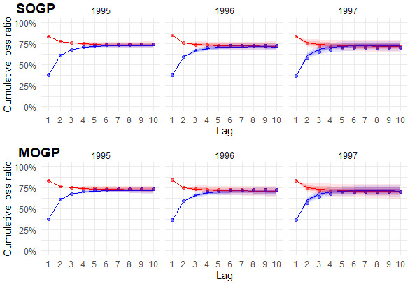
The predictions of the SOGP and MOGP models are similar, though the MOGP introduces a slightly higher level of uncertainty. This is most noticeable during the initial lags of the incurred pattern for accident year 1997. One potential explanation for the incurred pattern is the MOGP’s use of the sum of paid and case loss ratio predictions, as opposed to directly including incurred loss ratios in the model. Another factor affecting both loss types could be the MOGP’s ability to detect additional genuine uncertainty considering the interaction between triangles. An examination of results across a broader range of triangles in Section 5 may provide insight into which factor is more likely.

The most recent accident year, 1997, contributes the most to the total reserve estimate. The initial loss ratios for 1997 are similar to those of prior years, leading the models to predict a similar central estimate. However, in reality, the loss ratio developed lower than the recent history. Nonetheless, both the SOGP and MOGP models contained these loss ratios well within their predictive ranges.

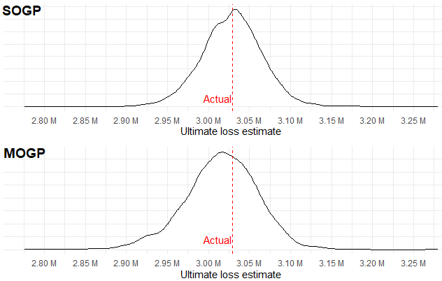
Figure 2 shows the estimate of ultimate loss across accident years. The predicted means of both models were close to the actual losses. The MOGP had slightly more variance in its prediction and a greater likelihood for lower reserves.

Figure 2.The predicted distributions of ultimate loss using the incurred projections at time 10.

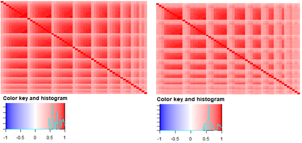
Like the predicted ranges, the model paths are largely similar. Both models find significant correlation between development lags and experience period loss ratios throughout the triangle. Figure 3 shows a median prediction of the training data correlation matrix for both incurred and paid loss ratios across accident years for the SOGP.

Figure 3.The left square represents incremental incurred loss ratio correlations for the training data. The right relates to incremental paid loss ratios. Within each matrix, the oldest accident year is in the top left, and the years progress along the diagonal, including their available development lags.

The two covariance matrices are largely similar. The main difference between the paid and incurred correlation matrices is the speed at which they reach correlations near 1. The incurred pattern, as expected, increases faster toward high correlation between development periods. The paid pattern finds weaker relationships in the first few development periods. Less correlation or higher noise increases the reliance on the mean vector, which is subjectively chosen and may not provide the best possible estimate.

The MOGP covariance matrix is displayed in Figure 4. The relationship between paid and case loss ratios is negative, as expected. Compared to the SOGP, correlation across development periods increases faster within the paid triangles. This may suggest we are relying less on the mean vector and improving the use of the available data after incorporating cross-triangle relationships. The cross-correlation terms exhibit similar patterns related to development and experience periods.

Figure 4.The incremental loss ratio correlations for the case loss ratios (top left), the paid loss ratios (bottom right), and the relationship between the two (bottom left and top right) for the training data. The oldest accident year is in the top left of each quadrant and the years progress along each diagonal including their available development lags.

The stronger correlation is also partially due to reduced noise in the MOGP model. Explicitly, the signal-to-noise ratio increases faster over the development periods compared with the SOGP models. Figure 5 shows the signal-to-noise ratio for each model and output. Drawing attention to the conclusions derived from the preceding figures, it is evident that both models identify similar patterns. However, the SOGP exhibits a greater degree of noise across the entire triangle, whereas the MOGP diminishes noise and leverages the available data more effectively, resulting in a broader spectrum of developmental patterns.

Figure 5.The signal-to-noise ratio for the SOGP paid model, SOGP incurred model, and the MOGP model, including case and paid projections by development lag.

4.1.1. Potential for improvement

The SOGP and MOGP are highly flexible for fitting loss development triangles. With that flexibility, low volume or noisy data can lead to slow convergence, inaccurate point predictions, or excessive uncertainty. To reduce the chance of each of these outcomes, we can do the following: increase the amount of data with quarterly lags, increase the amount of data with hierarchical structure, or create a more informed prior structure.

Increasing the amount of data with quarterly lags has the simplest implementation. The shape of the development curve would become more apparent, and the noise vector would have more parameters to monotonically decrease. On the downside, quarterly lags may dramatically increase run time depending on the number of experience years.

Alternatively, a hierarchical structure using multiple triangles of the same loss type (or group of loss types for the MOGP) could be constructed in two ways. The traditional approach would be to allow each triangle to fit its own GP using prior ranges informed by all triangles. This would demand slight changes in the prior structure defined in this paper. Another approach would be to model a set of kernels of which each triangle could determine weights. This would reduce the number of parameters estimated in the model and help the user discover underlying trends across the triangles. If the triangles chosen to model together are also expected to have a correlated structure, the LMC could be used to further support trend detection.

And lastly, a more informed prior structure could force what we’ve learned from a larger dataset onto the smaller. For instance, we could set a smaller prior range on signal variances within an experience period, especially as it approaches large development lags. This may be effective, but the user should be careful not to suppress reasonable uncertainty or real differences between triangles.

5. Performance testing

Retrospective testing for development methods on the NAIC dataset is well established to assess point and distribution estimates (Meyers 2015), and our metrics are borrowed directly from that framework. We repurpose open-source functions provided in Ludkovski and Zail (2021) to ensure comparable metrics across methods. Note that we copy the Ludkovski and Zail (LZ) results directly from their tables due to run time. Throughout, the LZ model will have one additional triangle in other liability (othliab) that was removed from the other methods due to having negative incurred loss, which disrupts the Mack chain ladder. Overall, this has no impact on relative model performance conclusions.

The following point accuracy metrics will be reviewed by line, loss ratio type, and premium group:

• Root mean squared error: $\sqrt{\frac{\sum_{t\epsilon T}^{\mathstrut}\left( C_{t,10} - {\widehat{C}}_{t,10} \right)^{2}}{\sum_{t\epsilon T}^{\mathstrut}1}}$

• Weighted root mean squared error: $\sqrt{\frac{\sum_{t\epsilon T}^{\mathstrut}\left( \frac{C_{t,10} - {\widehat{C}}_{t,10}}{P_{t}} \right)^{2}}{\sum_{t\epsilon T}^{\mathstrut}1}}$

In the preceding, $t$ is a triangle within the set of triangles $T$, $C_{t,10}$ is the sum of triangle $t$’s cumulative loss at lag 10, and $P_{t}$ is the total premium of a triangle $t$. $\widehat{C}$ is the model prediction of cumulative loss. The weighted root mean squared error (RMSE) is the more interpretable result (Ludkovski and Zail 2021) since one or a few large carriers can dominate the RMSE.

The following distribution metrics will be reviewed by line and loss ratio type:

• Coverage: A coverage metric evaluates the proportion of the data captured by a given probability distribution. We’ll test coverage of the middle 90%. A metric value near 0.90 suggests a good fit, while lower values suggest insufficient variance is captured by the model and higher values suggest excess variance is captured.

• Continuous rank probability score (CRPS): The CRPS is the squared difference between the predicted cumulative distribution function (CDF) and the actual distribution of observations. This provides information about the accuracy of the full probability distribution. We compare the sum of the squared differences across NAIC triangles. A lower CRPS indicates a better fit.

• Negative log probability density (NLPD): The NLPD measures the quality of a probability density estimate. It compares the estimated density with the true density of the data, with a lower NLPD indicating a better fit. This approach penalizes models that assign low probabilities to the observed data. This is commonly used to determine the best model for a given dataset. We compare the sums of NLPDs across NAIC triangles.

• Kolmogrov-Smirnov (K-S) statistic: The K-S statistic is the maximum absolute difference between an empirical distribution $F_{n}(x)$ and another $F(x)$. We will use an empirical CDF from our actual cumulative losses and compare it with the estimated CDF from the MOGP. The null hypothesis is that the samples come from the same distribution. We reject this hypothesis at the 5% level if the statistic exceeds $\frac{136}{\sqrt{n}}.$ In other words, the lower the K-S statistic, the better.

Reviewing these metrics together should help us achieve a comprehensive understanding of how well each model fits the data. We will confirm our insights by reviewing P-P plots and histograms of predicted and observed ultimate loss percentiles.

5.1. Point accuracy

The MOGP shows strong accuracy results on paid cumulative losses relative to other methods but generally underperforms the Mack chain ladder on incurred losses. Table 2 provides both accuracy metrics by line and in total. Emphasis is added to the top model for each line, metric, and loss type.

The initial conclusion for the MOGP is that shared learning seems to benefit the point prediction of paid dollars. Incorporating the incremental incurred loss ratios into the MOGP in addition to the case ratios may further improve the predictions.

Relative to other GP models, the MOGP produced consistently stronger results across all lines of business, while the SOGP generally outperforms all but the MOGP. The weighted RMSE metric clearly shows this, while the unweighted metric is more susceptible to distortion from a single data point. For example, one triangle contributes nearly 80% of the MOGP’s error for private passenger auto paid losses. As an alternative, we can review our weighted metric by premium group.

Table 3 provides the weighted accuracy metric split by premium group, and the results are consistent with prior conclusions. The unweighted metric is not included because the loss amounts would be dominated by private passenger auto.

The SOGP and MOGP both improve their relative performance as the volume of a triangle grows, showing their ability to better capture trends or understand patterns in the data. For small triangles such as those with less than $10 million in premium, we can pursue alternatives to increase the amount of data in the model (see Section 4.1.1).

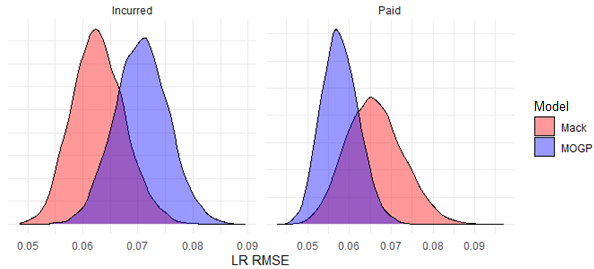
In Figure 6, we resample the weighted squared errors of the MOGP and Mack chain ladder model to produce distributions around the total for each. This further strengthens our conclusion that the accuracy of the selected MOGP model in predicting incurred losses is likely inferior to that of the Mack model, while it is expected to perform better in predicting paid losses.

Figure 6.Bootstrap distributions of weighted RMSE by loss type and model.

5.2. Distribution quality

The SOGP and MOGP produces strong distributional fits on ultimate losses relative to the other methods. Table 4 shows the distributional accuracy metrics for commercial auto triangles. Emphasis is added to the top performer for the CRPS and NLPD metrics, while values indicating the failure to reject the K-S null hypothesis are italicized.

The MOGP model exhibits a potential underfitting issue with incurred losses, while providing a reasonable distribution around paid losses. To address this, incorporating incremental incurred losses directly into the MOGP, instead of summing the predictions of paid and case losses, may improve the distributional fit.

In comparison with the SOGP, the MOGP consistently improves all distributional metrics for paid losses across lines of business (see Appendix C). Furthermore, the MOGP tends to display a wider range of total paid losses. This suggests that shared learning in the MOGP helps to uncover additional uncertainty or potential development patterns that may not be considered in a single-output model.

The MOGP struggled on the K-S test and coverage statistic in private passenger auto and workers compensation for paid triangles. This is generally due to the actual losses coming in below the median of our predicted distributions. There are a few possible explanations for this.

First, the model may be relying too much on prior lag development. If there is insufficient data in surrounding experience periods for a particular development lag, the model will more likely continue the development seen within the experience period to that point. When projecting paid development, that means we would more likely overstate ultimate losses.

Second, there may be insufficient data to pick up meaningful vertical trends. Like the first consideration, the model may not trust meaningful trends that are detected with only a few data points. This is a good feature as it may avoid overfitting, but following the ideas in Section 4.1.1 to expand the dataset can be considered.

Lastly, there may be additional factors not considered or easily detected in our data that are affecting development. A more advanced model can consider additional variables to adjust for known legal or underwriting changes, for example. The NAIC dataset we are using shows a disproportionate amount of low loss ratios in the more recent years. This suggests the existence of larger industry or economic variables affecting results that the current models are not able to recognize and extrapolate. Modeling mean vector adjustments related to external variables by experience period is a possible solution.

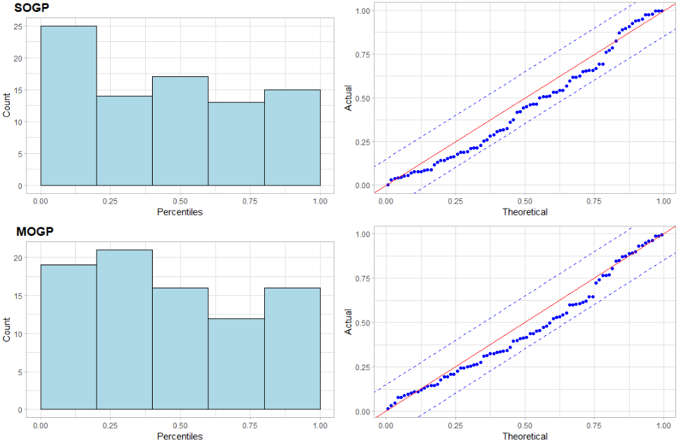
Figure 7 displays histograms and P-P plots for SOGP and MOGP models using commercial auto triangles. This shows how they may generally overstate paid losses. The actual percentiles are overrepresented below the theoretical line.

Figure 7.Histograms (left) and P-P plots (right) of cumulative paid loss percentiles for commercial auto triangles. The dotted lines represent the deviation necessary to reach K-S critical values.

Considering our coverage metric across lines of business, it seems that directly modeling the signal and noise variance and its relationship with development lag for both triangle dimensions is sufficient in capturing uncertainty in incurred patterns but may be insufficient for some paid patterns. Future improvements may scale the noise variance with relative experience period premium size or include another source of uncertainty.

6. Conclusion

The MOGP for loss development is a flexible time series model actuaries can use to estimate the distribution of ultimate loss reserves for multiple triangles. Using an additive kernel of the two triangle dimensions, we can increase parameter complexity and use multiple loss types with reasonable run times. The MOGP simultaneously learns incremental paid and case loss ratio patterns, improving the paid point predictions and estimates of uncertainty. Testing on the NAIC dataset shows arguably the best public model results to date.

The presented model is suited to estimate and share information across any number of loss ratio triangles. This may include ratios based on claim type, jurisdiction, or coverage code, for example. The main barrier is computational tractability. To overcome this, a variational inference procedure may be developed.

GPs are highly customizable and can account for many time series patterns and sources of uncertainty. They continue to be a strong framework for considering loss reserve models. The MOGP is another step toward an accurate, general development model for all lines of insurance.

Acknowledgment

I want to thank the anonymous reviewers for their time and consideration.