Gini Score Under Ties and Case Weights

1. Introduction

The Gini score is a popular statistical tool in model validation that was originally introduced and used for binary responses (i.e., $Y \in \{0,1\}$). The binary Gini score has many equivalent formulations, such as the receiver operating characteristics curve and the area under the curve (see, e.g., Bamber 1975; Hanley and McNeil 1982; Fawcett 2006). These different formulations are also equivalent to the Wilcoxon–Mann–Whitney $U$ statistic (Hanley and McNeil 1982; DeLong et al. 1988; Byrne 2016), and to Somer’s d (see Somers 1962; Newson 2002). Thus, the binary Gini score has at least five equivalent formulations, and its behavior is well understood and supported by a broad base of research literature.

However, with general real-valued responses, things become more difficult. In this context, Gini score definitions and results are found mainly in the credit risk and actuarial literature, where it was introduced by Gourieroux and Jasiak (2007), Frees et al. (2011; 2013), and studied in much detail by Denuit et al. (2019) and Denuit and Trufin (2021).

The Gini score assesses whether a given risk ranking is correct. Assume that we have a sample $(Y_i,\mu_i, \widehat{\mu}_i)_{i=1}^n$ with true means ${\mathbb E}[Y_i]=\mu_i$ and the corresponding estimates $\widehat{\mu}_i$, for $1\le i \le n$. In this case, the Gini score assesses whether the true means $(\mu_i)_{i=1}^n$ and their estimates $(\widehat{\mu}_i)_{i=1}^n$ provide the same risk ranking, where the maximal Gini score is attained if both risk rankings are identical. Thus, the Gini score is a purely rank-based concordance statistic and does not assess whether the estimated levels $(\widehat{\mu}_i)_{i=1}^n$ are correct. In particular, the shifted estimates $(a+\widehat{\mu}_i)_{i=1}^n$, for $a \in {\mathbb R}$, provide the identical risk ranking and therefore have the same Gini score. Even if we do not have the correct levels (also called calibration), assessing the risk ranking is often of central interest because, e.g., the correct risk ranking is a crucial assumption for applying an isotonic regression. For example, see Wüthrich and Ziegel (2024); also, the universal inference calibration test of Delong and Wüthrich (2025) is based on the assumption that the risk ranking is correct.

The Gini score, as introduced by Denuit et al. (2019), is based on the standard assumption that the risk ranking comprises a continuous random variable, which implies that a risk ranking has no ties $(\widehat{\mu}_i)_{i=1}^n$. However, many practical applications have tied estimates $(\widehat{\mu}_i)_{i=1}^n$. For example, if these estimates have been generated by gradient boosting machines, the very nature of their construction through regression trees will produce ties in the resulting risk rankings. Similarly, large insurance portfolios are likely to have multiple insurance policyholders with the same covariates and will therefore receive the same prediction for their claims. In such cases, ties in the samples will naturally occur; therefore, the classical Gini score needs to be adapted to handle these ties.

Our two main contributions are as follows: (1) We discuss the treatment of ties in the risk scoring. The handling of ties is surprisingly sensitive, so its treatment is crucial in a proper model selection process. (2) We discuss how to handle case weights. Responses are often supported by varying case weights (e.g., claims frequencies come together with time exposures). We discuss how such exposures and case weights can be integrated into Gini scores in the model selection process.

Organization. The Gini score is built on two different curves, the Leimkuhler curve that builds the denominator of the Gini score and the concentration curve (cumulative accuracy profile) that builds the numerator of the Gini score. The Leimkuhler curve is a mirrored version of the classical Lorenz curve. We discuss the Lorenz and Leimkuhler curves and the treatment of risk ranking ties in Section 2 and discuss the concentration curve in Section 3. Section 4 discusses the situation of including case weights, and Section 5 presents a real data example based on claims frequencies, which naturally include exposures (case weights). Section 6 summarizes our conclusions.

2. The Lorenz and Leimkuhler Curves

The Gini score is motivated by an economic concept introduced by Gini (1912; 1936). Based on the Lorenz curve (Lorenz 1905), the score measures wealth distribution disparities within a given population, where higher Gini scores indicate greater inequalities in wealth distribution. This concept was adapted for predictive modeling by measuring how well a given regression function discriminates responses. Here, we introduce the Lorenz (Lorenz 1905) and Leimkuhler curves, before diving into the Gini scoring in the next section.

2.1. Leimkuhler Curve

Select a nonnegative random variable $Y \sim F_Y$ with positive finite first moment ${\mathbb E}[Y]\in (0,\infty)$. The Lorenz curve is given by the function

$$\alpha \in (0,1)~ \mapsto ~ \frac{1}{{\mathbb E}[Y]} \,{\mathbb E}\left[ Y \,\mathbb{1}_{\{Y \le F_Y^{-1}(\alpha)\}}\right],\tag{2.1}$$

(see Denuit et al. 2019, Definition 3.2), where $F_Y^{-1}$ is the left-continuous generalized inverse of the distribution $F_Y$, given by

$$F_Y^{-1}(\alpha) = \inf \left\{ y \in {\mathbb R};\, F_Y(y)\ge \alpha \right\}.$$

For the machine learning version of the Gini score, we use the mirrored version of the Lorenz curve (the upper tail), known as the Leimkuhler curve (see Sarabia 2008). It is given by

$$\small{ \begin{align} \alpha \in (0,1)~ \mapsto ~ L_Y(\alpha) &= \frac{1}{{\mathbb E}[Y]} \,{\mathbb E}\left[ Y \,\mathbb{1}_{\{Y > F_Y^{-1}(1-\alpha)\}}\right] \\ &= 1- \frac{1}{{\mathbb E}[Y]} \,{\mathbb E}\left[ Y \,\mathbb{1}_{\{Y \le F_Y^{-1}(1-\alpha)\}}\right]. \end{align} \tag{2.2}}$$

The Leimkuhler curve (2.2) considers the order from the largest to the smallest observation, while the Lorenz curve (2.1) considers the opposite direction from the smallest to the largest observation. We calibrate the Leimkuhler curve $L_Y(\cdot)$ at the boundary of the open interval $(0,1)$ to $L_Y(0)=0$ and $L_Y(1)=1$.

Example 2.1 (continuous example). We consider a continuous distribution example. Assume that the random variable $Y$ has a lognormal distribution $\log(Y) \sim {\cal N}(m, \sigma^2)$. Its inverse is given by

$$F_Y^{-1}(1-\alpha) = \exp \left(m + \sigma \Phi^{-1}(1-\alpha)\right),$$

where $\Phi$ is the standard Gaussian distribution. In the lognormal case, the Leimkuhler curve is given by

$$\small{ \begin{align} \alpha \in (0,1)~ \mapsto ~ L_Y(\alpha) &= 1- \Phi \left(\frac{\log \left(F_Y^{-1}(1-\alpha)\right) - (m+\sigma^2)}{\sigma}\right) \\&= 1- \Phi \left( \Phi^{-1}(1-\alpha) - \sigma\right), \end{align}}$$

(see Cowell 2011, Section A.3.1). Note that the choice of parameter $m \in {\mathbb R}$ does not affect the Leimkuhler curve.

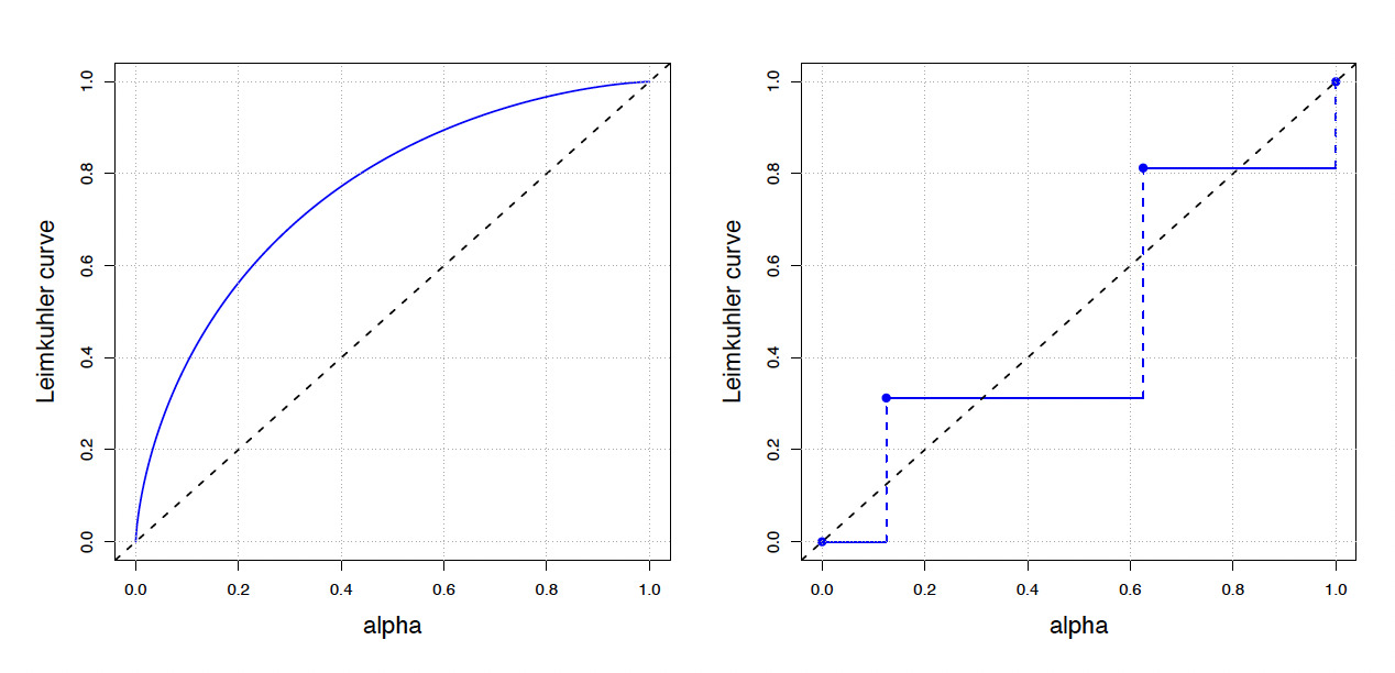
The Leimkuhler curve of this lognormal example is illustrated in Figure 1 (left panel) for $\sigma=1$. ∎

Figure 1.Leimkuhler curve: Lognormal case with $\sigma=1$ (left), discrete example (right).

Example 2.2 (discrete example). We consider a discrete example. Assume that the random variable $Y$ takes the following three values

$$Y = \left\{ \begin{array}{ll} 1/2 & \text{ with probability $p_1=3/8$,}\\ 1 & \text{ with probability $p_2=1/2$,}\\ 5/2 & \text{ with probability $p_3=1/8$.} \end{array} \right.\tag{2.3}$$

This random variable has an expected value ${\mathbb E}[Y]=1$ and its distribution $F_Y$ is a step function with steps in $y_k\in \{1/2,1,5/2\}$ having step sizes $p_k\in \{3/8,1/2,1/8\}$, for $k=1,2,3$. We compute the left-continuous generalized inverse for $p \in (0,1]$

$$F_Y^{-1}(p) = \left\{ \begin{array}{ll} 1/2 & \text{ for $p \in (0,3/8]$,}\\ 1 & \text{ for $p \in (3/8,7/8]$,}\\ 5/2 & \text{ for $p \in (7/8,1]$.} \end{array} \right.$$

This gives us the Leimkuhler curve

$$\begin{align} \alpha \in [0,1]~ \mapsto ~ L_Y(\alpha)&= \sum_{k=1}^3 p_k \, y_k\, \mathbb{1}_{\{y_k > F_Y^{-1}(1-\alpha)\}} \\&= \left\{ \begin{array}{ll} 0 & \text{ for $\alpha \in [0,1/8)$,}\\ 5/16 & \text{ for $\alpha \in [1/8,5/8)$,}\\ 13/16 & \text{ for $\alpha \in [5/8,1)$,}\\ 1 & \text{ for $\alpha=1$.} \end{array} \right. \end{align}$$

This Leimkuhler curve is illustrated in Figure 1 (right panel), and we notice that it is a step function in this discrete case. ∎

Examples 2.1 and 2.2 show two exact examples computed from the true distribution $F_Y$ of the response $Y$. In the next step, we consider the situation where the true distribution is unknown and we are only equipped with an independent and identically distributed (IID) sample $(Y_i)_{i=1}^n$ that has been generated from $F_Y$. This allows us to define the empirical distribution

$$\widehat{F}_n(y) = \frac{1}{n}\, \sum_{i=1}^n \mathbb{1}_{\{ Y_i \le y \}}, \qquad \text{ for $y \in {\mathbb R}$.}$$

The Glivenko–Cantelli result tells us that the empirical distribution $\widehat{F}_n$ converges to the true distribution $F_Y$ uniformly, a.s., that is, $\lim_{n\to \infty}\|\widehat{F}_n-F_Y\|_\infty=0$, a.s. This justifies taking the empirical distribution as an approximation to the true one (for large $n$). This empirical distribution allows us to estimate the Leimkuhler curve $L_Y$ by its empirical counterpart

$$\begin{align} \alpha &\in (0,1)~ \mapsto ~ \widehat{L}_n(\alpha) \\&= \frac{1}{\frac{1}{n}\sum_{i=1}^n Y_i}\, \frac{1}{n}\, \sum_{i=1}^n Y_i \,\mathbb{1}_{\{Y_i > \widehat{F}_n^{-1}(1-\alpha)\}}. \end{align}\tag{2.4}$$

Again, we set the boundary of the unit interval $\widehat{L}_n(0)=0$ and $\widehat{L}_n(1)=1$. This gives us a step function analogous to Example 2.2, with step sizes determined by the observations $(Y_i)_{i=1}^n$.

In case of no ties in the observations, we can build the strict order statistics $Y_{(1)}>\ldots > Y_{(n)}$, and all step heights in the empirical distribution $\widehat{F}_n$ are equal to $1/n$. This allows expressing the empirical Leimkuhler curve by (in the case without ties)

$$\begin{align} \alpha &\in (0,1)~ \mapsto ~ \widehat{L}_n(\alpha) \\&= \frac{1}{\frac{1}{n}\sum_{i=1}^n Y_i}\, \frac{1}{n}\, \sum_{i=1}^{n-\lceil (1-\alpha)n\rceil} Y_{(i)}, \end{align}\tag{2.5}$$

where an empty sum is set equal to zero.

Example 2.3 (continuous example: empirical version). We revisit the lognormal case of Example 2.1, which has a continuous distribution, so we cannot have ties in the observed sample $(Y_i)_{i=1}^n$. Therefore, formula (2.5) applies.

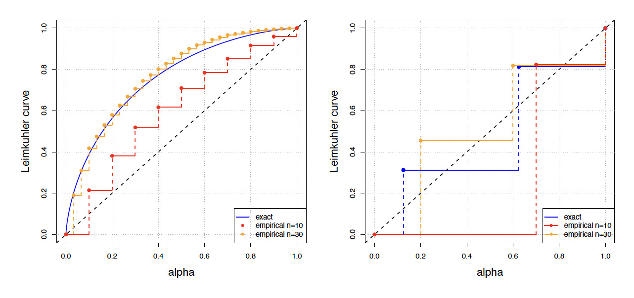
Figure 2 (left panel) gives two empirical examples of different sample sizes $n=10,30$ (red, orange). Naturally, if we resample the observations $(Y_i)_{i=1}^n$, we get different results (on finite samples), but the results converge to the true Leimkuhler curve, a.s., as the sample size goes to infinity. ∎

Figure 2.Empirical Leimkuhler curve for sample sizes $n=10,30$ (red, orange): Empirical lognormal case (left), empirical discrete case (right).

Example 2.4 (discrete example: empirical version). We revisit the discrete Example 2.2 and simulate two samples of size $n=10,30$ from the true discrete distribution (2.3). Figure 2 (right panel) shows the results. The smaller sample contains only two labels $\{1/2, 1\}$, and we obtain a step function with two steps for the empirical Leimkuhler curve $\widehat{L}_n$. In the larger sample, all three labels $\{1/2, 1, 5/2\}$ occur, and the empirical Leimkuhler curve begins to approximate the true curve more closely. These empirical Leimkuhler curves were calculated from formula (2.4). ∎

2.2. Linearly Interpolated (Empirical) Leimkuhler Curve

Figure 2 shows that the (empirical) Leimkuhler curve can be both above and below the diagonal dashed line. For the Gini score introduced in Section 3, it is beneficial to have a curve that does not fall below the diagonal dashed line to allow computing the area enclosed by that curve and the diagonal dashed line. In the noncontinuous case, this can be achieved by a linear interpolation between the discrete points (instead of a step function interpolation). Assume that we have an IID sample $(Y_i)_{i=1}^n$ from a distribution $F_Y$ (this sample may have ties). Assume that this sample takes $K$ unique values $(Y^\star_k)_{k=1}^K$. This allows us to define the aggregated case weights in these unique values

$$w_k^\star = \frac{1}{n}\,\sum_{i=1}^n \mathbb{1}_{\{Y_i = Y^\star_k\}}, \qquad \text{ for $k=1, \ldots, K$.}$$

These aggregated case weights precisely describe the step heights in the empirical distribution of $(Y_i)_{i=1}^n$. That is, we have two equivalent versions of the empirical distribution

$$\widehat{F}_n(y) = \frac{1}{n}\, \sum_{i=1}^n \mathbb{1}_{\{ Y_i \le y \}} =\sum_{k=1}^K w_k^\star\, \mathbb{1}_{\{ Y^\star_{k} \le y \}}.$$

Consider strict order statistics $Y^\star_{(1)} > \ldots >Y^\star_{(K)}$, and map the identical ordering to the case weights $(w^\star_{[k]})_{k=1}^K$, using square bracket notation to indicate that this is implied by the order statistics of the responses. The steps on the $x$-axis in the empirical graphs in Figure 2 are precisely in the points

$$\alpha^\star_k = \sum_{j=1}^k w^\star_{[j]}, \qquad \text{ for $k=1, \ldots, K$,}$$

and we initialize $\alpha^\star_0=0$. The incremental step heights of the empirical Leimkuhler curve (on the $y$-axis) in these steps are given by

$$\frac{1}{\sum_{j=1}^K w^\star_{[j]} Y^\star_{(j)}} \, w^\star_{[k]} Y^\star_{(k)},$$

and in the aggregated version they are equal to

$$\widehat{L}_n(\alpha^\star_k) =\frac{1}{\sum_{j=1}^K w^\star_{[j]} Y^\star_{(j)}} \, \sum_{j=1}^k w^\star_{[j]} Y^\star_{(j)} , \qquad \text{ for $k=0, \ldots, K$.}$$

The orange and red dots in Figure 2 illustrate this set, called the corner set

$${\cal B}^\star=\left(\alpha^\star_k, \,\widehat{L}_n(\alpha^\star_k)\right)_{k=0}^K.\tag{2.6}$$

We now linearly interpolate between these points in the corner set ${\cal B}^\star$; that is, for $\alpha \in (\alpha^\star_{k-1}, \alpha^\star_k]$, $k=1, \ldots, K$, we set

$$\begin{align} \widehat{L}^+_n(\alpha) &= \widehat{L}_n(\alpha^\star_{k-1}) \\&\quad+ \frac{\widehat{L}_n(\alpha^\star_k)-\widehat{L}_n(\alpha^\star_{k-1})}{\alpha^\star_k-\alpha^\star_{k-1}}\left(\alpha - \alpha^\star_{k-1}\right). \end{align}\tag{2.7}$$

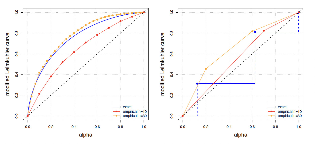
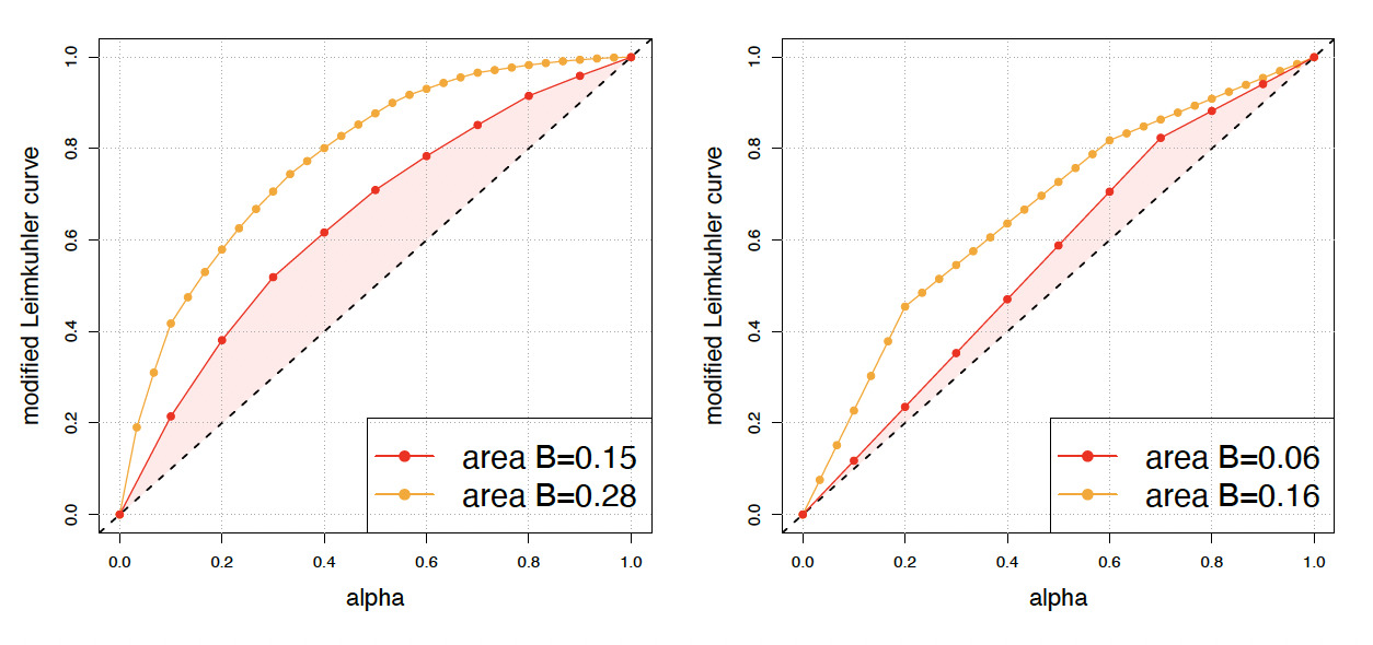
We call this linearly interpolated version the modified empirical Leimkuhler curve. Naturally, this concept can be applied to any discrete distribution, not only to the empirical one. The results of this linear interpolation in the empirical cases are shown by the red and orange graphs in Figure 3 (the true discrete distribution in blue is not linearly interpolated in this graph).

Figure 3.Modified (linearly interpolated) empirical Leimkuhler curve $\widehat{L}_n^{+}$ for sample sizes $n=$ 10, 30: Lognormal case (left), discrete case (right)

This linear interpolation comes with several advantages:

1. The aggregation over the unique values in the sample $(Y_i)_{i=1}^n$ is not necessary (i.e., in the case of ties, they automatically enter correctly into the modified Leimkuhler curve). We can build order statistics $Y_{(1)}\ge \ldots \ge Y_{(n)}$, with a deterministic rule in the ties. This allows us to consider the modified empirical Leimkuhler curve in the values $\alpha_i=i/n$ for $i\in \{0,\ldots, n\}$
   $$\widehat{L}^+_n(\alpha_i) =\frac{1}{\frac{1}{n}\sum_{j=1}^n Y_j} \, \frac{1}{n}\sum_{j=1}^i Y_{(j)},\tag{2.8}$$
   where the empty sum is set equal to zero. This gives us the corner set
   $${\cal B}=\left(\alpha_i=\frac{i}{n}, \,\widehat{L}^+_n(i/n)\right)_{i=0}^n.\tag{2.9}$$
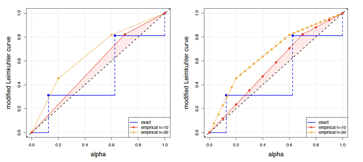
   Linear interpolation over this corner set ${\cal B}$ produces a curve that is identical to the modified empirical Leimkuhler curve (2.7). Figure 4 verifies that both versions—the aggregated tie and the nonaggregated tie—give the same piecewise linear graph. Thus, aggregation in the ties is not necessary if we interpolate linearly over the corner set ${\cal B}$.

Figure 4.Modified empirical Leimkuhler curve $\widehat{L}_n^{+}$ in the discrete case: Constructed on the aggregated order statistics $\left(Y_{(k)}^{\star}\right)_{k=1}^K$ with corner set $\mathcal{B}^{\star}$ (left) and on the nonaggregated order statistics $\left(Y_{(i)}\right)_{i=1}^n$ with corner set $\mathcal{B}$ (right). The two red areas are identical.

2. The dashed diagonal now receives an explicit meaning: If all observations are identical, $Y_1=\ldots = Y_n$, the diagonal gives the modified empirical Leimkuhler curve, and whenever there are at least two different observations $Y_j\neq Y_k$ for some $j\neq k$, the modified empirical Leimkuhler curve $\widehat{L}^+_n$ lies above the dashed diagonal.

3. The area between the modified empirical Leimkuhler curve $\widehat{L}^+_n$ and the diagonal is always a convex set, and its area is strictly positive when there are at least two different observations in the sample $(Y_i)_{i=1}^n$. This is implied by the corner sets being constructed from decreasing order statistics and is verified in Figure 4 by the red area that illustrates the smaller sample with $n=10$.

In view of the last item in the list of advantages of the modified empirical Leimkuhler curve, we can also easily compute the resulting convex area implied by the corner set ${\cal B}$ (above the diagonal). Based on (2.8) and (2.9), we compute the size of the enclosed convex area by

$$\small{\begin{align}B := \sum_{i=1}^n \frac{\widehat{L}^+_n(\alpha_i) + \widehat{L}^+_n(\alpha_{i-1})}{2}\, \left(\alpha_i - \alpha_{i-1}\right) - \frac{1}{2}.\end{align}\tag{2.10}}$$

The size of this area is indicated in the graph legend in Figure 5 and is illustrated by the red area in the case of the smaller samples $n=10$ (in red).

Figure 5.Modified empirical Leimkuhler curve $\widehat{L}_n^{+}$ showing the area $B$ that is enclosed in the convex set between the diagonal dashed line and the modified empirical Leimkuhler curve $\widehat{L}_n^{+}$ for sample sizes $n=10,30$ : Lognormal case (left), discrete case (right).

3. Cumulative Accuracy Profile

3.1. The Continuous Distribution Case

We start from a random triplet $(Y,\mu,\widehat{\mu})$ characterizing an insurance policyholder, which has the following interpretation: First, we randomly select an insurance policyholder from the insurance portfolio by simulating their average claim $\mu \sim {\mathbb P}$ from the portfolio (population) distribution ${\mathbb P}$; second, we simulate the claim $Y$, given $\mu$, satisfying the calibration property

$$\mu={\mathbb E}\left[ \left. Y \right| \mu \right], \qquad \text{a.s.}\tag{3.1}$$

Thus, $\mu$ reflects the conditionally expected claim of $Y$ and provides the correct risk ranking in terms of conditionally expected claims. Finally, we determine (simulate) the estimated claim $\widehat{\mu}$ and assume that $Y$ and $\widehat{\mu}$ are conditionally independent, given $\mu$. This conditional independence reflects the fact that we perform an out-of-sample model evaluation. We summarize these assumptions in the model as follows.

Assumptions 3.1. Assume the random triplet $(Y,\mu,\widehat{\mu})$ has the following structure:

• (1) Calibration: $\mu={\mathbb E}[Y| \mu]$, a.s., with integrable mean ${\mathbb E}[|\mu|]<\infty$.
• (2) Out-of-sample evaluation: $Y$ and $\widehat{\mu}$ are conditionally independent, given $\mu$.

We can now simulate an IID sample $(Y_i,\mu_i, \widehat{\mu}_i)_{i=1}^n$ under Assumptions 3.1, which provides a true risk ranking $(\mu_i)_{i=1}^n$ and an estimated risk ranking $(\widehat{\mu}_i)_{i=1}^n$. The main question we would like to study with the Gini score is whether these two risk rankings coincide (i.e., are concordant). We give some preliminary remarks.

Remarks 3.2

• Assumptions 3.1 give the full modeling setup. In insurance applications, we are only equipped with an observed IID sample $(Y_i,\widehat{\mu}_i)_{i=1}^n$. The true means $(\mu_i)_{i=1}^n$ are unknown, so we must estimate them, and we would like to determine whether the estimates $(\widehat{\mu}_i)_{i=1}^n$ provide the correct risk ranking. We try to answer this question empirically by using the responses $(Y_i)_{i=1}^n$ that have been generated from these unknown means $(\mu_i)_{i=1}^n$.

• Calibration. In the considerations below, $\mu$ describes the true conditional mean providing (3.1). For the risk ranking analysis, it is only important to know the correct ordering. That is, we may start from any risk ranking $\pi=g(\mu)$, with a strictly increasing function $g$, then $\mu$ and $\pi$ provide the same risk ranking, and they generate the same $\sigma$-field—in fact, they are strictly comonotonic. Consequently, the isotonic recalibration step promoted in Wüthrich and Ziegel (2024), Section 3.1, then provides the true conditional mean
  $$\mu={\mathbb E}\left[ \left. Y \right| \pi \right], \qquad \text{a.s.}$$
  Thus, knowing the correct risk ranking $\pi$, the true means $\mu$ can be inferred by this isotonic recalibration step.

• Out-of-sample evaluation. The response $Y$ and the estimate $\widehat{\mu}$ are assumed to be conditionally independent, given $\mu$. Unconditionally, they should have a positive association, otherwise clearly, $\widehat{\mu}$ will not be suitable to describe the risk ranking.

• In insurance applications, $\mu=\mu(\pmb{X})$ reflects the true regression function on the covariates $\pmb{X}$, and $\widehat{\mu}=\widehat{\mu}(\pmb{X})$ its estimated counterpart, which has been estimated on an independent learning sample ${\cal L}$. In this setup, the simulation process of Assumptions 3.1 is changed to simulate an insurance policyholder with covariates $\pmb{X}\sim {\mathbb P}$. This gives the true regression function $\pmb{X}\mapsto \mu(\pmb{X})={\mathbb E}[Y|\pmb{X}]$, which fulfills calibration (3.1). We then assess whether the estimated regression function $\pmb{X}\mapsto \widehat{\mu}(\pmb{X})$ gives the correct risk ranking; the dependence between $Y|_{\pmb{X}}$ and $\widehat{\mu}(\pmb{X})$ is implied because both random variables are considered under the identical covariate $\pmb{X}$.

The cumulative accuracy profile (CAP) modifies the Leimkuhler curve as follows:

$$\begin{align}\alpha &\in (0,1)~ \mapsto ~ C_{\mu, \widehat{\mu}}(\alpha) \\&= \frac{1}{{\mathbb E}[\mu]} \,{\mathbb E}\left[ \mu \,\mathbb{1}_{\{\widehat{\mu} > F_{\widehat{\mu}}^{-1}(1-\alpha)\}}\right].\end{align}\tag{3.2}$$

At the boundary of the unit interval, we set $C_{\mu, \widehat{\mu}}(0)=0$ and $C_{\mu, \widehat{\mu}}(1)=1$. This is the mirrored version of the concentration curve of Denuit et al. (2019, Definition 3.1). The CAP describes an asymmetric concordance function (i.e., we aggregate the true means $\mu$ in the decreasing order of their estimated counterparts $\widehat{\mu}$). The more the ordering between $\mu$ and $\widehat{\mu}$ are aligned, the larger the resulting CAP, and in the perfect ordering case, we precisely obtain the Leimkuhler curve $L_\mu(\alpha)=C_{\mu, \mu}(\alpha)$. Thus, we have

$$C_{\mu, \widehat{\mu}}(\alpha) \le L_\mu(\alpha), \qquad \text{ for all $\alpha \in [0,1]$,}$$

with an equality if $\widehat{\mu}$ and $\mu$ are comonotonic.

As explained in the first item of Remarks 3.2, in insurance applications the true means $\mu$ are unknown, only observations $Y$ generated from these means are available. This requires us to study a different version of the CAP.

Lemma 3.3. Under Assumptions 3.1, we have for all $\alpha \in [0,1]$

$$C_{\mu, \widehat{\mu}}(\alpha) = C_{Y, \widehat{\mu}}(\alpha) = \frac{1}{{\mathbb E}[Y]} \,{\mathbb E}\left[ Y \,\mathbb{1}_{\{\widehat{\mu} > F_{\widehat{\mu}}^{-1}(1-\alpha)\}}\right].$$

Assume $g$ is a strictly increasing function. Then, $C_{Y, g(\widehat{\mu})}(\alpha)=C_{Y, \widehat{\mu}}(\alpha)$ for all $\alpha\in [0,1]$.

Proof. The first statement is an immediate consequence of the model assumptions and the tower property of conditional expectations by conditioning on $(\mu,\widehat{\mu})$. The second statement immediately follows from the two sets $\{\widehat{\mu} > F_{\widehat{\mu}}^{-1}(1-\alpha)\}=\{g(\widehat{\mu}) > F_{g(\widehat{\mu})}^{-1}(1-\alpha)\}$ being equal for any strictly increasing function $g$. ∎

The first part of Lemma 3.3 tells us that, based on an observed IID sample $(Y_i,\widehat{\mu})_{i=1}^n$, the CAP can be evaluated empirically. The second part says that the CAP is a purely rank-based measure in $\widehat{\mu}$ (which does not consider calibration). Moreover, (3.3) and Lemma 3.3 imply that

$$\int_{0}^1 C_{Y, \widehat{\mu}}(\alpha) \,\mathrm{d}\alpha \le \int_{0}^1 L_{Y}(\alpha)\, \mathrm{d}\alpha.\tag{3.4}$$

This inequality (3.4) is the core of the Gini score defined below.

We now estimate the CAP from an IID sample $(Y_i,\widehat{\mu}_i)_{i=1}^n$ under Assumptions 3.1, additionally assuming that $\widehat{\mu}$ has a continuous distribution $F_{\widehat{\mu}}$. The latter implies that $(\widehat{\mu}_i)_{i=1}^n$ does not have ties, and we obtain the strict order statistics $\widehat{\mu}_{(1)}>\ldots >\widehat{\mu}_{(n)}$. We map the identical ordering to the responses $(Y_{[i]})_{i=1}^n$ using square bracket notation (i.e., the ordering of the responses is implied by the ranking of the estimates), $(\widehat{\mu}_{(i)})_{i=1}^n$. This motivates the empirical CAP

$$\begin{align}\alpha &\in (0,1)~ \mapsto ~ \widehat{C}_n(\alpha) \\&= \frac{1}{\frac{1}{n}\sum_{i=1}^n Y_i}\, \frac{1}{n}\, \sum_{i=1}^{n-\lceil (1-\alpha)n\rceil} Y_{[i]},\end{align}\tag{3.5}$$

with initializations $\widehat{C}_n(0)=0$ and $\widehat{C}_n(1)=1$. The main difference between (2.5) and (3.5) is that the former takes the order statistics of the responses $(Y_i)_{i=1}^n$ and the latter takes the order statistics of the estimates $(\widehat{\mu}_i)_{i=1}^n$.

This empirical CAP is a step function, which allows us to consider a piecewise linear modification. Similarly to (2.8), define the corner set

$$\small{{\cal A}= \left( \alpha_i=\frac{i}{n}, ~ \widehat{C}^+_n(i/n) =\frac{1}{\frac{1}{n}\sum_{j=1}^n Y_j} \, \frac{1}{n}\sum_{j=1}^i Y_{[j]}\right)_{i=1}^n,\tag{3.6}}$$

and linearly interpolate between these corners to produce the modified empirical CAP $\alpha \mapsto \widehat{C}^+_n(\alpha)$ on $[0,1]$. Analogously to (2.10), this allows us to compute the area

$$\small{A := \sum_{i=1}^n \frac{\widehat{C}^+_n(\alpha_i) + \widehat{C}^+_n(\alpha_{i-1})}{2}\, \left(\alpha_i - \alpha_{i-1}\right) - \frac{1}{2}.\tag{3.7}}$$

The estimated Gini score divides the area implied by the corner set ${\cal A}$ (see (3.7)) by the area implied by the corner set ${\cal B}$ (see (2.10)), resulting in

$$\operatorname{Gini}(Y_i,\widehat{\mu}_i)_{i=1}^n ~:= ~ \frac{A}{B} ~\le ~1.\tag{3.8}$$

For (3.8) we assume that at least two observations in $(Y_i)_{i=1}^n$ differ, which implies $B>0$, and the upper bound is given by the Leimkuhler curve considering the perfect ordering, which is achieved if the ranks of the responses $(Y_i)_{i=1}^n$ and the estimates $(\widehat{\mu}_i)_{i=1}^n$ are aligned.

→ This solves the case of estimates $(\widehat{\mu}_i)_{i=1}^n$ without ties.

Remark 3.4. The Gini score denominator ($B$) is strictly positive as soon as the observations have at least two different values. The Gini score numerator ($A$) can have any sign. Assume that the predictions $(\widehat{\mu}_i)_{i=1}^5=(1,2,3,4,5)$ are strictly increasing and the corresponding responses are strictly decreasing $(Y_i)_{i=1}^5=(5,4,3,2,1)$; this reflects a counter-monotonic setting. In this case, we obtain a modified empirical CAP that lies below the diagonal, hence $A<0$.

3.2. The Noncontinuous Distribution Case

If the distribution $F_{\widehat{\mu}}$ is not continuous, the estimates $(\widehat{\mu}_i)_{i=1}^n$ are likely to have ties, and we do not receive a unique ordering.

Q: How should we deal with ties in $(\widehat{\mu}_i)_{i=1}^n$?

First answer. Taking inspiration from the nonempirical version (3.2), we simply aggregate in the ties. Assume that we have $K$ unique values $(\widehat{\mu}^\star_k)_{k=1}^K$ in $(\widehat{\mu}_i)_{i=1}^n$. This motivates the aggregate case weights

$$w_k^\star = \sum_{i=1}^n \frac{1}{n}\,\mathbb{1}_{\{\widehat{\mu}_i = \widehat{\mu}^\star_k\}}, \qquad \text{ for $k=1, \ldots, K$,}$$

and the average observation (empirical mean)

$$\begin{align} Y_k^{\star}&=\frac{1}{w_k^{\star}} \sum_{i=1}^n Y_i \frac{1}{n} \mathbb{1}_{\left\{\widehat{\mu}_i=\widehat{\mu}_k^{\star}\right\}}, \quad \text { for } \\ k&=1, \ldots, K . \end{align}\tag{3.9}$$

We can apply this process to the new sample $(Y^\star_k,\widehat{\mu}^\star_k, w^\star_k)_{k=1}^K$, which does not have ties in $(\widehat{\mu}^\star_k)_{k=1}^K$. (For the case weights, we refer to Section 4).

However, we argue that this process is not a good option for dealing with ties. Typically, the goal is to assess the risk rankings of different predictive models $(\widehat{\mu}^{(1)}_i)_{i=1}^n$ and $(\widehat{\mu}^{(2)}_i)_{i=1}^n$. By aggregating the ties (3.9) of the two models, the models may benefit differently from the law of large numbers. The following example illustrates this.

Example 3.5 (aggregation in ties). Assume that we have the following responses

$$\small{(Y_1,Y_2,Y_3,Y_4, Y_5,Y_6, Y_7,Y_8)=(1.99,2,3,4, 5, 6, 7, 8).}$$

These responses have the property that the first two are difficult to distinguish, and the remaining responses are well separated. Assume that we have two models for the estimates such that

$$\small{\left(\widehat{\mu}^{(1)}_1, \widehat{\mu}^{(1)}_2, \widehat{\mu}^{(1)}_3, \widehat{\mu}^{(1)}_4, \widehat{\mu}^{(1)}_5, \widehat{\mu}^{(1)}_6, \widehat{\mu}^{(1)}_7, \widehat{\mu}^{(1)}_8\right) = \left(2.01,2,3,4, 5, 6, 7, 8 \right),}$$

and

$$\small{\left(\widehat{\mu}^{(2)}_1, \widehat{\mu}^{(2)}_2, \widehat{\mu}^{(2)}_3, \widehat{\mu}^{(2)}_4, \widehat{\mu}^{(2)}_5, \widehat{\mu}^{(2)}_6, \widehat{\mu}^{(2)}_7, \widehat{\mu}^{(2)}_8\right) = \left(3,3,3,3,7,7,7,7 \right).}$$

The first model ($\widehat{\mu}^{(1)}$) produces a perfect ranking except for the first two responses that are difficult to distinguish. In fact, it slightly overestimates the smallest observed response. The second model ($\widehat{\mu}^{(2)}$) can only rank better (3) from worse (7) (i.e., the estimates are binary), and most will agree that the first model does a better job of risk ranking because the second is a crude binary model.

Using averaging (3.9) for the second model with ties, we get

$$\begin{align} (Y^\star_1,Y^\star_2)&=(2.7475, 6.5) \qquad \text{ and } \\ ((\widehat{\mu}^{(2)})^\star_1, (\widehat{\mu}^{(2)})^\star_2) &= (3,7). \end{align} \tag{3.10}$$

Thus, on the aggregated scale, the second model provides a perfect ranking. Naturally, we should not compare the aggregated statistics of the second model with the nonaggregated statistics of the first model, because the coarser model benefits more from averaging (3.9)—a law of large numbers. In other words, for model comparison and selection we should consider both models on the same granularity. ∎

We conclude from Example 3.5 that we should not aggregate in the ties of $(\widehat{\mu}_i)_{i=1}^n$ but always consider the models on an identical observation scale to produce a fair comparison.

Note that in many applied situations, the estimated regression models do not have the same granularity (e.g., when constructing two different gradient boosting machine estimators that differ only in, say, the choices of tree size or their shrinkage factors, they will likely have a different granularity).

Second answer. Instead of aggregating in the ties of $(\widehat{\mu}_i)_{i=1}^n$, we use the original observation scale with sample size $n$. Consider the order statistics $\widehat{\mu}_{(1)}\ge \ldots \ge \widehat{\mu}_{(n)}$, which in the case of ties does not give a unique ranking. We map this ranking to the responses $(Y_i)_{i=1}^n$, and in the ties of $(\widehat{\mu}_{i})_{i=1}^n$ we take two extreme positions where $(Y_{[i\downarrow]})_{i=1}^n$ is the ordered sample that uses the same ordering as the order statistics of $(\widehat{\mu}_{i})_{i=1}^n$, and in the ties of $(\widehat{\mu}_{i})_{i=1}^n$, the responses are in decreasing order (that is, we use the responses for a suborder in the ties). For the second extreme case, we let $(Y_{[i\uparrow]})_{i=1}^n$ have an increasing suborder in the ties of $(\widehat{\mu}_{i})_{i=1}^n$ with respect to the responses. This gives us two samples $(Y_{[i\downarrow]})_{i=1}^n$ and $(Y_{[i\uparrow]})_{i=1}^n$ that are ordered with respect to the order statistics of $(\widehat{\mu}_{i})_{i=1}^n$, and in its ties we use the responses $(Y_i)_{i=1}^n$ for a suborder (requiring a deterministic rule if the responses also have ties in the ties of the estimates).

Analogously to (3.6), we define the two corner sets ${\cal A}^\downarrow$ and ${\cal A}^\uparrow$ by setting $\alpha_i=i/n$, for $i\in \{0,\ldots, n\}$, and

$$\begin{align} \widehat{C}^\downarrow_n(\alpha_i) &=\frac{1}{\frac{1}{n}\sum_{j=1}^n Y_j} \, \frac{1}{n}\sum_{j=1}^i Y_{[j\downarrow]} \qquad \text{ and }\\ \widehat{C}^\uparrow_n(\alpha_i) &=\frac{1}{\frac{1}{n}\sum_{j=1}^n Y_j} \, \frac{1}{n}\sum_{j=1}^i Y_{[j\uparrow]}. \end{align}$$

An easy consequence of the selected suborders in the ties is that

$$\widehat{C}^\downarrow_n(\alpha_i) \ge \widehat{C}^\uparrow_n(\alpha_i), \qquad \text{ for all $i\in \{0,\ldots, n\}$.}$$

Obviously, any other suborder in the ties is between these two bounds. $\widehat{C}^\downarrow_n$ represents a best case CAP, because the ordering within the ties is optimal with respect to the responses, and $\widehat{C}^\uparrow_n$ represents the worst case CAP (with the least optimal ordering in the ties). In a binary context, this corresponds to Fawcett (2006, Figure 6).

Figure 6.Gini score evaluated on a sample size of $n=20$ : First model $\widehat{\mu}^{(1)}$ (left), second model $\widehat{\mu}^{(2)}$ (right).

Because we want a single Gini score at the end, we define the mid-solution in $\alpha_i=i/n$ for $i\in \{0,\ldots, n\}$ by

$$\small{ \begin{align} \widehat{C}^+_n(\alpha_i) &= \frac{1}{2}\left(\widehat{C}^\downarrow_n(\alpha_i)+ \widehat{C}^\uparrow_n(\alpha_i)\right) \\&= \frac{1}{\frac{1}{n}\sum_{j=1}^n Y_j} \, \frac{1}{n}\sum_{j=1}^i \frac{1}{2}\left(Y_{[j\downarrow]}+ Y_{[j\uparrow]}\right), \end{align} \tag{3.11}}$$

and it is linearly interpolated between these points.

Remarks 3.6.

• The mid-solution in the binary context presented in Fawcett (2006, Figure 6), differs from our proposal in that it does not consider a suborder in the ties implied by the responses but connects the corner set obtained from the unique values $(\widehat{\mu}^\star_k)_{k=1}^K$ by straight lines. This can be interpreted as an expected sorting because any observation within a tie occurs with the same probability, and averaging over all permutations gives a straight line instead of suborders in ties. Our mid-solution (3.11) generally does not give a straight line in the ties. However, we prove in Lemma 3.7 that both solutions, the straight line of Fawcett (2006) and our mid-solution (3.11), lead to an identical Gini score value (3.13) (i.e., the geometric objects are different, but they include the same area).

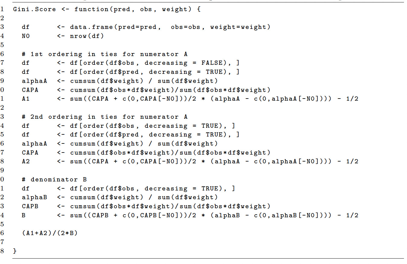
• We prefer our solution because it is computationally more appealing. It does not require explicitly identifying the ties, but it can be implemented by first ordering for $(Y_i)_{i=1}^n$ and then for $(\widehat{\mu}_i)_{i=1}^n$. The second sorting typically keeps the order of the first one in the ties. This then gives the correct order for aggregating to receive the CAP. A code example is given in Listing 1 in the Appendix.

• Both our solution with suborders in the ties and the straight line solution of Fawcett (2006) have an advantage over a random ordering in the ties in that they provide a unique (and replicable) value. Therefore, we do not recommend a random ordering in the ties (as is sometimes done in practice).

• In relation to the last item, where a constant prediction $\widehat{\mu}_i\equiv \widehat{\mu}$ produces one big tie, our mid-solution provides the diagonal line, which results in a Gini score of zero in (3.13), below.

• The best case CAP $\widehat{C}^\downarrow_n$ and the worst case CAP $\widehat{C}^\uparrow_n$ are identical in the case where all observations in the ties are identical. This is particularly the case for the Leimkuhler curve that enters the denominator of the Gini score (see (3.13)). Therefore, with the Leimkuhler curve, we do not need to consider the best and worst cases, but we can directly interpolate by straight lines (see Figure 4).

The mid-solution is identical to (3.6) in the case without ties and extends to the case with ties in the estimates $(\widehat{\mu}_i)_{i=1}^n$. Analogously to (3.7), we define in this more general case the area induced by these corner points

$$\small{A = \sum_{i=1}^n \frac{\widehat{C}^+_n(\alpha_i) + \widehat{C}^+_n(\alpha_{i-1})}{2}\, \left(\alpha_i - \alpha_{i-1}\right) - \frac{1}{2}.\tag{3.12}}$$

The estimated Gini score is defined by

$$\operatorname{Gini}(Y_i,\widehat{\mu}_i)_{i=1}^n ~=~ \frac{A}{B} ~\le~ 1.\tag{3.13}$$

For two models, $\widehat{\mu}^{(1)}$ and $\widehat{\mu}^{(2)}$, the second model provides the more accurate risk ranking measured by the Gini score if

$$\operatorname{Gini}(Y_i,\widehat{\mu}^{(1)}_i)_{i=1}^n ~\le ~ \operatorname{Gini}(Y_i,\widehat{\mu}^{(2)}_i)_{i=1}^n ~\le ~ 1.$$

Lemma 3.7. Consider the aggregated sample $(Y_k^\star, \widehat{\mu}_k^\star, w_k^\star)_{k=1}^K$ such that $(\widehat{\mu}_k^\star)_{k=1}^K$ does not have ties. Similarly to (4.4) and (4.5), below, this leads to a corner set ${\cal A}$ without ties. By connecting this set of corners with straight lines we can compute the area enclosed by the diagonal line that results precisely in the value $A$ given in (3.12).

This lemma states that our mid-solution (3.12) and the straight line solution in the binary case of Fawcett (2006) produce the same Gini score (see also Remarks 3.6).

Proof of Lemma 3.7. Consider the suborders $(Y_{[i\downarrow]})_{i=1}^n$ and $(Y_{[i\uparrow]})_{i=1}^n$ in the ties, which precisely reflect the Leimkuhler curve (2.2) and the Lorenz curve (2.1), respectively. Consequently, the enclosed areas of these two curves with the diagonal line are the same, but with opposite signs. Therefore, if we average these two areas, we obtain the same area as the one computed from the diagonal straight line, thus proving the claim. ∎

Example 3.8 (Gini score under ties). We consider two examples with ties. We assume that the true mean $\mu$ has a uniform distribution over the set

$$\left\{1,2,3,8,9,10 \right\},$$

and we simulate the response by a conditional Gaussian distribution $Y|\mu \sim {\cal N}(\mu,1)$. We assume that we have two different estimates (models) $\widehat{\mu}^{(1)}$ and $\widehat{\mu}^{(2)}$ being deterministic functions of $\mu$, described by the following ordered samples

$$\begin{gathered} \mu = 1,2,3,8,9,10 & \Longrightarrow & \widehat{\mu}^{(1)}=1,2,3,10,7,8,\\ \mu = 1,2,3,8,9,10 & \Longrightarrow & \widehat{\mu}^{(2)}=2,2,2,10,7,8. \end{gathered}$$

That is, the first model $\widehat{\mu}^{(1)}$ has the correct risk ranking in the lowest three values but incorrectly allocates the highest risk 10 to position 4. The second model $\widehat{\mu}^{(2)}$ has the same wrong ordering of the three largest risks and cannot distinguish the three smallest risks. From this we conclude that the first model ($\widehat{\mu}^{(1)}$) should be preferred over the second ($\widehat{\mu}^{(2)}$) with respect to the risk ranking.

The previous conclusion uses the knowledge of the true mean $\mu$, which in practical problems is not available, and we try to match this conclusion from a validation sample. Therefore, we generate an IID sample $(Y_i,\mu_i,\widehat{\mu}_i)_{i=1}^n$ from this model of sample size $n=20$.

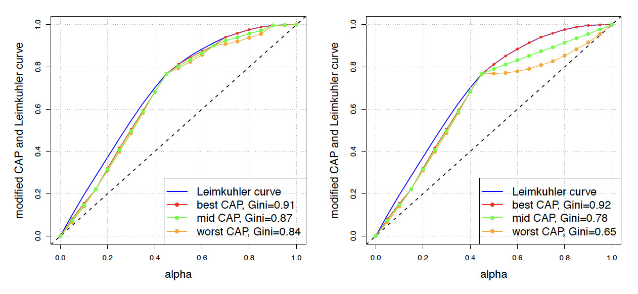
The results of the two estimated models $\widehat{\mu}^{(1)}$ and $\widehat{\mu}^{(2)}$ are shown in Figure 6 (left and right panels, respectively). The blue curve shows the modified (linearly interpolated) Leimkuhler curve (2.8)–(2.9), which determines the denominator $B$ of the Gini score (see (2.10)). The red and orange curves are the best CAP $\widehat{C}^\downarrow_n$ and the worst CAP $\widehat{C}^\uparrow_n$, respectively, and the green line gives the mid-solution CAP $\widehat{C}^+_n$, see (3.11), which is used to compute the numerator $A$ of the Gini index (see (3.12) and (3.13)). This results in Gini scores

$$\operatorname{Gini}(Y_i,\widehat{\mu}^{(1)}_i)_{i=1}^n =0.87 ~> ~ \operatorname{Gini}(Y_i,\widehat{\mu}^{(2)}_i)_{i=1}^n =0.78.$$

Thus, we conclude from these Gini scores that the first model $\widehat{\mu}^{(1)}$ gives the more accurate risk ranking, which is the same conclusion we drawn above.

An important insight from Figure 6 is that we have also computed Gini scores if we focus on the best CAPs $\widehat{C}^\downarrow_n$ for the two models (red graphs in the two plots). We note that this best CAP would give an incorrect preference to the second model that cannot correctly distinguish the lower three risk rankings because the equal scores give a bigger tie in the second model $\widehat{\mu}^{(2)}$ compared with the first model $\widehat{\mu}^{(1)}$. Using the optimal suborder in this tie gives an unjustified preference to the second model (Gini score 0.92 versus 0.91 in the first model). The effect here is similar to the law of large numbers effect (3.10), which suggests that for model selection we should use the mid-solution (3.11) to ensure that both models are judged using the same granularity. ∎

The implementation of our mid-solution (3.12) is straightforward (see Listing 1 in the Appendix). Using standard software requires care because some of these tools consider the best case CAP, which is not fully suitable (as argued in the previous example).

4. Case Weights

Insurance data often include so-called case weights. In fact, an insurance policyholder is characterized by a random quadruplet $(Y,\mu,\widehat{\mu},w)$. That is, the random triplet of Section 3.1 is extended by a positive case weight $w>0$ because insurance liabilities and insurance claims are often measured relative to an exposure measure, such as time, total insurance sum, building value, number of insured employees, etc. The frequency of claims provides a common case, where $Y$ models the frequency of claims and $wY$ is the total number of claims in an exposure period of length $w$. The prediction $\widehat{\mu}$ is then on the level of a premium rate, and $w\widehat{\mu}$ gives the effectively charged premium for the claim $wY$ in the time interval of length $w$.

From a modeling perspective, this is supported by the exponential dispersion family (EDF), which is the most popular class of distribution functions for regression modeling. Generalized linear models (GLMs) are based on the EDF, and the EDF contains many useful distribution functions, such as Gaussian, Poisson, negative binomial, gamma, inverse Gaussian, and Tweedie. The standard representation within the EDF is where $Y$ is a scaled quantity with case weight $w>0$, also known as the reproductive form of the random variable $Y$ (see Jørgensen (1997) and Wüthrich and Merz (2023)).

With an IID sample $(Y_i,\mu_i,\widehat{\mu}_i,w_i)_{i=1}^n$, we may analyze the problem of a correct risk ranking analogously to that of Section 3. However, should we perform the risk ranking in the scaled $Y$ or the unscaled $wY$ version? If we perform this risk ranking in the unscaled version, we consider the case weight-adjusted IID sample $(w_iY_i,w_i\mu_i,w_i\widehat{\mu}_i)_{i=1}^n$. Based on this unscaled IID sample, we proceed according to Section 3.

We argue in favor of the scaled version $(Y_i,\mu_i,\widehat{\mu}_i,w_i)_{i=1}^n$. Often, case weights $w_i$ are deterministic quantities that are fixed in insurance contracts at the time of inception. For example, we may have a small company that wants to purchase accident insurance for its $w_1=100$ workers, and we may have a big company that wants to purchase accident insurance for its $w_2=1{,}000$ workers. Under the assumption that the claims ratios $\mu_i$ do not depend on the case weights, we should charge the first company $w_1 \mu_1$ and the second company $w_2 \mu_2$. Assuming that the second company’s business is more prone to accidents (e.g., office work versus construction work), we then assume $\mu_1 = 1$ and $\mu_2=2$ (i.e., $\mu_1 < \mu_2$). Thus, the true means $(\mu_i)_{i=1}^n$ describe the correct claim propensities, which must be scaled by the size (volume) of the respective insurance contract. Assume in the previous example that we have predictors $\widehat{\mu}_1 = 1.75$ and $\widehat{\mu}_2=1.50$, providing the wrong risk ranking $\widehat{\mu}_1>\widehat{\mu}_2$. This incorrect risk ranking will be overruled in the unscaled case by including the case weights (i.e., $w_1\widehat{\mu}_1=175<w_2\widehat{\mu}_2=1{,}500$), and we will not detect that our tariff scheme $(\widehat{\mu}_i)_{i=1}^n$ does not match the correct risk ranking of the true means $(\mu_i)_{i=1}^n$. Therefore, we prefer scaled quantities $(Y_i,\mu_i,\widehat{\mu}_i,w_i)_{i=1}^n$ because they bring us closer to the ground truth of the true means $(\mu_i)_{i=1}^n$.

Integrating the case weights into the Gini score is done by replacing the identical empirical weights of one by the corresponding case weights. In the first step, we compute the denominator of the Gini score by modifying the corner set ${\cal B}$ given in (2.9) as follows: Build the order statistics $Y_{(1)} \ge \ldots \ge Y_{(n)}$ on the scaled responses and define its implied order $(w_{[i]})_{i=1}^n$ on the case weights. On the $x$-axis of the Leimkuhler curve, we set $i \in \{0, \ldots, n\}$

$$\alpha_i = \frac{1}{ \sum_{j=1}^n w_j}\, \sum_{j=1}^i w_{[j]},\tag{4.1}$$

and on the $y$-axis

$$\widehat{L}^+_n(\alpha_i) =\frac{1}{\sum_{j=1}^n w_jY_j} \, \sum_{j=1}^i w_{[j]} Y_{(j)}.\tag{4.2}$$

This gives us a new corner set ${\cal B}=(\alpha_i, \,\widehat{L}^+_n(\alpha_i))_{i=0}^n$ for the weighted quantities. By linear interpolation, we compute the denominator of the Gini score by

$$B = \sum_{i=1}^n \frac{\widehat{L}^+_n(\alpha_i) + \widehat{L}^+_n(\alpha_{i-1})}{2}\, \left(\alpha_i - \alpha_{i-1}\right) - \frac{1}{2}.\tag{4.3}$$

Naturally, this includes (2.10) using the specific choice $w_i\equiv 1$.

For the numerator of the Gini score, we consider the order statistics $\widehat{\mu}_{(1)}\ge \ldots \ge \widehat{\mu}_{(n)}$, and in the case of ties, we use the best and worst suborder implied by the responses $(Y_i)_{i=1}^n$. This implies labeling of the responses $(Y_{[i\downarrow]})_{i=1}^n$ and $(Y_{[i\uparrow]})_{i=1}^n$, and we map this ordering also to the case weights $(w_{[i\downarrow]})_{i=1}^n$ and $(w_{[i\uparrow]})_{i=1}^n$. Next, we define the two corner sets ${\cal A}^\downarrow$ and ${\cal A}^\uparrow$ by setting

$$\begin{align} \alpha^\downarrow_i &= \frac{1}{ \sum_{j=1}^n w_j}\,\sum_{j=1}^i w_{[j\downarrow]} \qquad \text{ and }\\ \alpha^\uparrow_i &= \frac{1}{ \sum_{j=1}^n w_j}\,\sum_{j=1}^i w_{[j\uparrow]}, \end{align}\tag{4.4}$$

for $i\in \{0,\ldots, n\}$, and

$$\begin{align} \widehat{C}^\downarrow_n(\alpha^\downarrow_i) &=\frac{1}{\sum_{j=1}^n w_jY_j} \, \sum_{j=1}^i w_{[j\downarrow]}Y_{[j\downarrow]} \qquad \text{ and }\\ \widehat{C}^\uparrow_n(\alpha^\uparrow_i) &=\frac{1}{\sum_{j=1}^n w_jY_j} \, \sum_{j=1}^i w_{[j\uparrow]}Y_{[j\uparrow]}. \end{align}\tag{4.5}$$

Again, we initialize these quantities to zero in zero and to one in one. This gives us the best- and worst-case areas, respectively,

$$\small{ A^{\downarrow}=\sum_{i=1}^n \frac{\widehat{C}_n^{\downarrow}\left(\alpha_i^{\downarrow}\right)+\widehat{C}_n^{\downarrow}\left(\alpha_{i-1}^{\downarrow}\right)}{2}\left(\alpha_i^{\downarrow}-\alpha_{i-1}^{\downarrow}\right)-\frac{1}{2}, \tag{4.6}}$$

$$\small{ A^{\uparrow}=\sum_{i=1}^n \frac{\widehat{C}_n^{\uparrow}\left(\alpha_i^{\uparrow}\right)+\widehat{C}_n^{\uparrow}\left(\alpha_{i-1}^{\uparrow}\right)}{2}\left(\alpha_i^{\uparrow}-\alpha_{i-1}^{\uparrow}\right)-\frac{1}{2} . \tag{4.7}}$$

The estimated Gini score under case weights is defined by

$$\operatorname{Gini}(Y_i,\widehat{\mu}_i, w_i)_{i=1}^n ~=~ \frac{(A^\downarrow+A^\uparrow)/2}{B} ~\le~ 1.\tag{4.8}$$

This coincides with (3.13) for identical case weights $w_i \equiv \text{constant}>0$. Note that we cannot directly merge the best and worst case corner sets of the CAP because the aggregated weights $(\alpha^\downarrow_i)_{i=1}^n$ and $(\alpha^\uparrow_i)_{i=1}^n$ may take different values on the $x$-axis. The code for (4.8) is given in Listing 1 in the Appendix.

5. Real Data Example

For this example, we used the well-known French third-party motor liability (MTPL) data set from Dutang et al. (2024). We considered the claim frequencies for $Y$ and used the same data cleaning and the same learning data and test data partition as described in Wüthrich and Merz (2023).^[1]

Data characteristics are shown in Table 1. We fitted two different GLMs on the learning dataset ${\cal L}$ using different sets of covariates: The first GLM (glm1) is a more granular regression model, and the second GLM (glm2) is a cruder regression model that only considers some covariates. Naturally, we expected the first GLM to provide a better risk ranking because it considers more (granular) covariate information. We fitted these two regression models on the learning sample ${\cal L}$, which provided the two regression functions

$$\pmb{X}\mapsto \widehat{\mu}^{\tt glm1}(\pmb{X}) \qquad \text{ and }\qquad \pmb{X}\mapsto \widehat{\mu}^{\tt glm2}(\pmb{X}).\tag{5.1}$$

All subsequent analysis was conducted on the test sample ${\cal T}$ only. Generally, model validation and selection should use an independent sample that has not been used for model fitting to avoid introducing an in-sample bias in the decision process. This also aligns with the conditional independence assumption of item (2) in Assumptions 3.1. Thus, we studied the risk rankings on the two test samples ${\cal T}^{\tt glm1}=(Y_i, \widehat{\mu}_i^{\tt glm1},w_i)_{i=1}^n$ and ${\cal T}^{\tt glm2}=(Y_i, \widehat{\mu}_i^{\tt glm2},w_i)_{i=1}^n$, where $(Y_i,w_i)$ are the out-of-sample observed frequencies and exposures of the test instances $i \in \{1,\ldots, n\}$ in ${\cal T}$ (see Table 1). The two predictors were obtained considering the previously fitted regression functions (5.1) on the out-of-sample instances with covariates $\pmb{X}_i$; that is,

$$\widehat{\mu}_i^{\tt glm1}:=\widehat{\mu}^{\tt glm1}(\pmb{X}_i) \qquad \text{ and }\qquad \widehat{\mu}_i^{\tt glm2}:=\widehat{\mu}^{\tt glm2}(\pmb{X}_i).$$

The out-of-sample Poisson deviance losses of the two models are given by

$$\begin{align} \text{Poisson deviance of $\widehat{\mu}^{\tt glm1}$}&=0.457 \qquad \text{ and } \\ \text{Poisson deviance of $\widehat{\mu}^{\tt glm2}$}&= 0.475. \end{align}$$

Thus, the first GLM clearly performed better in terms of the Poisson deviance loss. (For theoretical background on loss scoring we refer to Wüthrich et al. (2025), Formula 1.26 and Table 2.2.)

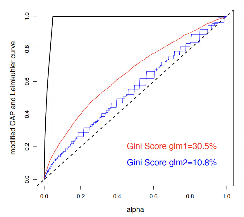
Our goal was to understand how these two models perform in terms of the risk ranking computed by the Gini score (being calculated out-of-sample on ${\cal T}$). We started by computing the Leimkuhler curve (4.1) and (4.2), which provides the denominator $B$ of the Gini score. We note that this MTPL claims frequency dataset faces the typical class imbalance, which means that insurance policies with zero claims $Y_i=0$ are much more common than policies with claims $Y_i>0$; this is also reflected in the low empirical frequency of roughly $7.35\%$ (see Table 1). This class imbalance results in a steep Leimkuhler curve until it reaches level one; then it is constantly equal to one (reflecting all insurance policies that do not suffer any claims; see the solid black curve in Figure 7). The thin black vertical dashed line

$$\frac{1}{\sum_{i=1}^n w_i} \sum_{i=1}^n w_i \,\mathbb{1}_{\{ Y_i>0\}}= 4.77\%$$

is the relative exposure of instances with claims.

Figure 7.French MTPL data: Out-of-sample Gini scoring of the two different GLMs: glm1 in red color and glm2 in blue color. The blue and red curves show the best and worst case CAPs; the black solid line gives the Leimkuhler curve.

Next, we calculate the empirical worst and best case CAPs (4.4) and (4.5), which provide the Gini score numerators $A^\downarrow$ and $A^\uparrow$. A consequence of class imbalance is that pure randomness (irreducible risk) dominates the systematic regression structure, typically resulting in out-of-sample losses dominated by irreducible risk. This also manifests itself in comparably small Gini scores measured by the observation version $C_{Y,\widehat{\mu}}(\alpha)$ of the CAP, because the randomness in $Y$ dominates this quantity. We computed the worst and best case CAP in both GLMs, glm1 and glm2, illustrated in red and blue in Figure 7, where glm2 (in blue) is a coarse-grained GLM having many ties in the predictions $\widehat{\mu}_i^{\tt glm2}$, resulting in CAP graphs that clearly distinguish the best from the worst case CAP (see Figure 7). For the fine-grained glm1 (in red), the differences are invisible because we have fewer (big) ties and the observations in the ties are more similar.

Computing the Gini score (4.8) from these graphs

$$\begin{align} \operatorname{Gini}(Y_i,\widehat{\mu}^{\tt glm1}_i, w_i)_{i=1}^n&=30.5\% \qquad \text{ and } \\ \operatorname{Gini}(Y_i,\widehat{\mu}^{\tt glm2}_i, w_i)_{i=1}^n&=10.8\%, \end{align}$$

we give clear preference to the first GLM in terms of the risk ranking (see the code in Listing 1). We emphasize that these quantities were calculated out-of-sample in the test set ${\cal T}$, while the learning set ${\cal L}$ was used solely to estimate the regression functions (5.1).

6. Conclusion

The Gini score is a popular tool for statistical modeling and machine learning model selection and validation. It is a purely rank-based score that assesses risk rankings; that is, it only assesses the risk rankings of predictions, not their levels (see Wüthrich (2023)). Typically, this Gini score assumes that the resulting risk ranking does not have ties. This paper discusses the treatment of ties and the consideration of additional case weights. For the ties, we considered two different suborders in the ties and averaged the two results to obtain a unique Gini score. The technical construction of this Gini score differs from that of the binary context straight line solution proposed by Fawcett (2006), but the resulting Gini score values are identical. Our second main takeaway is that when comparing risk rankings between two different models, their Gini scores should be computed with the same granularity; otherwise, one model may benefit more from the law of large numbers, which will result in incomparable Gini scores.