1. Introduction
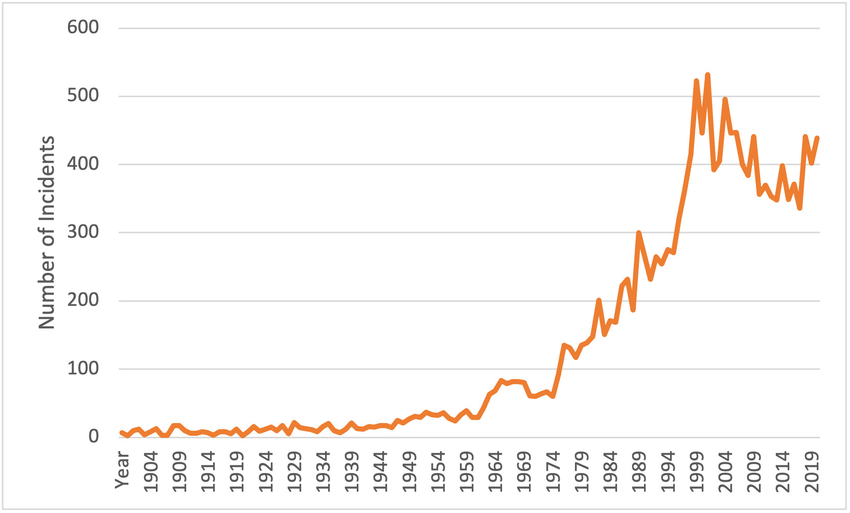
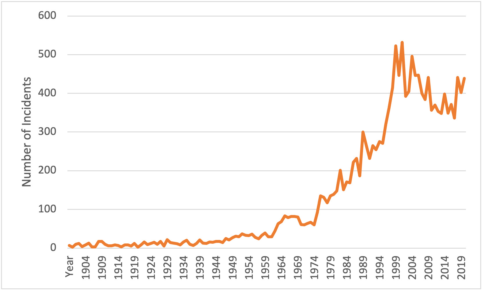
Catastrophic events—ranging from natural disasters to human-made crises—can cause severe damage to individuals, businesses, and entire communities. In recent years, global climate change has exacerbated climate variability and extreme weather events, leading to more frequent and costly natural disasters worldwide (Van Aalst 2006). As Figure 1 shows, the frequency of disasters has risen dramatically over recent decades. The heightened risks of catastrophic events, including tropical cyclones, droughts, floods, and heatwaves, pose unprecedented challenges to society’s resilience and adaptability. These challenges have made disaster risk mitigation and climate change adaptation strategies increasingly urgent (Mercer 2010).
The Intergovernmental Panel on Climate Change has underscored the necessity of financial instruments to manage disaster risk and support climate adaptation efforts (Linnerooth-Bayer and Hochrainer-Stigler 2015). Developing innovative tools for managing financial exposure to weather risks is crucial. The insurance sector has emerged as a pivotal player in protecting human, economic, and natural systems from climate-related vulnerabilities (Mills 2007; Keucheyan 2018). Within this context, catastrophe insurance serves as a vital risk management mechanism, not only providing financial support for post-disaster recovery but also creating incentives for proactive investment in mitigation efforts.
Catastrophe insurance, also known as disaster insurance, focuses on large-scale, low-frequency events that can cause widespread damage. It typically covers disasters such as hurricanes, earthquakes, floods, terrorist acts, and pandemics. The rarity of such catastrophic events complicates the insurance process, as traditional actuarial methods fall short, often due to a lack of comprehensive historical data. Compounding that challenge, climate change is leading to more regular and destructive climate-related catastrophes, which traditional reliance on historical data alone tends to underestimate. In contrast to conventional insurance policies that spread risks across insured individuals, catastrophe insurance confronts a temporal problem of matching the regular influx of annual premiums with the irregular and unforeseeable distribution of payouts for losses.
In the United States, catastrophe insurance has historically been managed predominantly through national programs. The National Flood Insurance Program (NFIP), for example, is the principal provider of flood insurance in the country, covering more than 95% of the underwriting risks (E. O. Michel-Kerjan 2010). However, the NFIP’s actuarial effectiveness has been the subject of scrutiny, with the program operating at a significant deficit—US$19 billion as of 2023—highlighting the need for reform in the structuring of such insurance schemes (Horn and Brown 2017). The entry of private insurers into the catastrophe coverage market has been deemed crucial, yet the inherent complexities associated with rare events have led to minimal participation from private entities (E. Michel-Kerjan and Kunreuther 2011). Indeed, many private insurers are withdrawing from regions deemed “uninsurable” due to escalating risks from climate change (Flavelle et al. 2023). Regulators and insurers are thus particularly concerned about insolvency risks in catastrophe insurance markets, as extreme events can trigger large-scale, correlated losses that threaten insurers’ financial stability. These solvency concerns have led to stringent capital requirements and risk transfer mechanisms, such as reinsurance and catastrophe bonds, to enhance the resilience of insurance providers (Charpentier and Le Maux 2014).
In this paper, we present an adaptive robust optimization (ARO) framework for catastrophe insurance premium pricing designed to protect against uncertain losses. To the best of our knowledge, this is the first work using an ARO approach to set disaster insurance premiums. We develop the framework and implement it to flood insurance using NFIP data. The main contributions are threefold:
-
We present an ARO framework designed for the pricing of catastrophe insurance premiums. The novel framework integrates two key objectives: minimizing insolvency risk and ensuring capital efficiency. Specifically, we develop an uncertainty set that captures the volatile loss profile based on historical loss distributions, enhancing insurers’ resilience against catastrophic events.
-
We apply our ARO framework to US flood insurance using data from the NFIP from 1975 to 2022. We parameterize optimization models using 1975–2011 data as training data and evaluate model performance using 2013–2022 data as out-of-sample testing data. Optimization models demonstrate capabilities in effectively covering losses while offering adaptability to policymakers’ risk tolerance and level of conservatism. In particular, we recommend that policymakers choose an ARO model, with conservative parameter values, to achieve superior performance in both effectiveness and efficiency in covering losses.
-
We highlight the adaptability and generalizability of our framework, suggesting the potential application of an ARO approach to pricing a wide range of catastrophic events, such as wildfires, droughts, and extreme weather events.
The structure of the paper is as follows. In Section 2, we review the relevant literature. In Section 3, we introduce the problem setup and present both the robust optimization (RO) and the ARO frameworks. We derive their respective robust counterparts in forms that can be efficiently solved using standard optimization solvers. In Section 4, we demonstrate the application of our framework through a case study on flood insurance in the United States. We explain model construction and model parameter estimation. In Section 5, we discuss numerical results of the case study from our models against two baselines: historical NFIP premiums and a cumulative moving average (CMA) scheme. Finally, we conclude in Section 6.
2. Literature review
The problem studied in this paper pertains to three key areas: (1) catastrophe insurance pricing, (2) catastrophe modeling, and (3) disaster relief planning. Our methodology builds on research in adaptive and robust optimization.
2.1. Catastrophe insurance pricing
The cost of catastrophe insurance comprises three key components: average annual loss (AAL), risk load, and expense load (Grossi 2005). AAL represents the total expected loss from all covered events within a year. The expense load accounts for administrative costs, including taxes, commissions, and loss adjustment expenses, typically set as a fixed percentage (e.g., 30%) of the combined AAL and risk load. Unlike conventional property and casualty insurance (e.g., auto insurance), where losses remain relatively stable across large pools and AAL constitutes the bulk of the premium, catastrophe losses are characterized by extreme volatility. Insurers need to allocate substantial additional capital beyond the expected loss to ensure that they can absorb rare shocks, and the risk load reflects such a cost premium.
To mitigate insolvency risks, regulators require insurers to adhere to capital adequacy principles, often through exceedance probability thresholds to ensure that the probability of total losses surpassing available capital remains acceptably low (Olivieri and Pitacco 2015). The required capital varies based on insurer-specific strategies and regulatory mandates (Jaffee and Russell 1997). For example, the Florida Office of Insurance Regulation stress-tests hurricane insurers to ensure that the probability of insolvency does not exceed 1% (Nicholson et al. 2018). Instead of decomposing risks into AAL and risk load, our approach adopts an optimization framework, directly modeling the cost required to prevent insolvency risk by constructing uncertainty sets around expected losses. This allows for a more flexible and robust risk assessment, accounting for volatility without relying solely on predefined risk load assumptions.
2.2. Catastrophe modeling
Catastrophe modeling, or CAT modeling, is a computational framework that integrates statistical, geophysical, and economic data to estimate the likelihood and financial impacts of extreme events such as hurricanes, earthquakes, and floods. Widely used by insurers and policymakers, CAT models assess disaster probabilities and estimate physical and financial losses (Grossi 2005). Modern CAT models consist of three key modules: hazard modeling, vulnerability assessment, and exposure modeling (Mitchell-Wallace et al. 2017). Hazard modeling simulates event characteristics (e.g., wind speed, earthquake magnitude) using statistical and physics-based methods, with machine learning improving predictive accuracy (Rueden et al. 2020; Chen and Zhang 2022). Vulnerability assessment quantifies the relationship between hazard intensity and damage, while exposure modeling links predicted damages to affected assets and populations through high-resolution geospatial and socioeconomic datasets. The market is dominated by proprietary models from AIR Worldwide, RMS, and EQECAT, alongside open-source alternatives like the Federal Emergency Management Agency’s (FEMA’s) HAZUS (Schneider and Schauer 2006).
Despite their widespread use, CAT models face challenges such as limited historical data, complexities in scenario simulations, and the underestimation of risks, particularly under climate change (Kunreuther et al. 2013; Dlugolecki et al. 2009). Emerging hybrid approaches that combine machine learning with physics-based models offer improved transparency, robustness, and adaptability (Zahura et al. 2020). This paper contributes to the literature by introducing an optimization-based framework that directly addresses uncertainties in losses and climate risks, enhancing tail-event risk assessment and improving decision-making for risk management.
2.3. Disaster relief planning
Many studies have focused on the problem of general resource allocations to different programs or regions under a given budget constraint (Wang et al. 2023; Alem et al. 2016; Salmerón and Apte 2010). Yang et al. (2021) discuss fund allocation for flash flood reduction, and Liu et al. (2022) further incorporate the use of insurance premiums as a source of funding. As highlighted by Kunreuther et al. (2013), the critical issue in insurance policy lies in the need for decision-making robustness in the face of climate change’s uncertainties. There is also a growing body of work on using robust optimization in disaster relief management to deal with uncertainties (Ben-Tal et al. 2011; Zokaee et al. 2016). Few studies discuss the use of optimization for catastrophe insurance pricing directly. Ermolieva et al. (2017) apply stochastic optimization to the Dutch flood insurance scheme. Our study fills in the gap by proposing a robust optimization framework by modeling uncertain losses to address the increasing unpredictability of weather events driven by climate change.
3. Optimization framework for catastrophe insurance
In this section, we introduce a realistic problem setup from the perspective of an insurer, where annual premium rates must be determined under significant uncertainty about future losses. Losses due to natural disasters and other extreme events are inherently uncertain, often exhibiting heavy tails, temporal variability, and limited data availability. To account for such uncertainty in a systematic and risk-averse manner, we adopt an RO framework. RO provides a natural approach for modeling uncertainty by optimizing decisions against the worst-case outcomes within a predefined uncertainty set, which is defined using historical loss distribution. We then present the robust counterpart of the RO formulation, which can be solved efficiently using standard optimization solvers. To further enhance flexibility, we introduce an ARO framework, which allows rate-setting decisions in future years to adapt to realized losses, reflecting the evolving information available to insurers over time. Finally, we derive the robust counterpart of the ARO formulation.
3.1. Problem setup
In this study, we consider setting insurance premiums for locations for the insurance period of years, denoting premiums as variables where Following industry practice, we assume that each location represents the smallest geographical unit where catastrophe risk has been assessed and that a standard premium is charged. We are given the data of historical losses for each location for each year in the past years, which we denote with , We assume that the future losses for each location in the insurance period of years are given by Future losses for location over the insurance period are inherently uncertain. However, to first establish our formulation framework, we assume knowledge of and later introduce an RO approach to systematically model this uncertainty.
The objective is to determine the minimum premium that will ensure financial stability while offering the most competitive rate in the market. This involves optimizing capital efficiency, specifically, covering insolvency risks with the least amount of required capital. By minimizing capital requirements, insurers are better positioned to lower premiums and remain competitive. To account for consumer behavior, where higher premiums lead to decreased demand, we introduce a demand-damping function which is a monotonically decreasing function representing the decline in demand as premiums increase. Therefore, the overall objective function of the optimization problem is as follows:
minpi,tN∑i=1T∑t=1f(pi,t)∗pi,t.
To model the damping behavior of demand as price increases, we adopt a piecewise linear function. This choice ensures that the resulting objective function remains quadratic in the premium variable preserving the tractability for most optimization solvers to find a solution efficiently. Moreover, the damping rate can be flexibly controlled through a tunable hyperparameter, allowing us to accurately reflect the sensitivity of demand to price changes.
Next, to protect insurers against insolvency risk, we require the premium price to cover projected losses with an additional buffer amount, denoted by which is a fixed threshold for each location. To ensure financial stability, then, premiums must exceed projected losses by the buffer amount, leading to the following constraint:
T∑t=1f(pi,t)∗pi,t−T∑t=1f(pi,t)∗li,t≥δ,i∈[N].
Next, we impose a constraint to require premiums collected over consecutive years to vary slowly. Insurance regulators typically impose limits on year-over-year premium increases to prevent market disruptions and financial strain on policyholders. Thus, we enforce the following constraint to require premiums collected in subsequent years to be bounded by an absolute value :
|pi,t−pi,t−1|≤θ,i∈[N],t∈[T].
Finally, should be nonnegative, for all locations over all periods, to ensure feasibility in all scenarios:
pi,t∈R+,i∈[N],t∈[T].
3.2. Robust optimization formulation
In our initial problem setup, we assume that projected future losses are known. However, in reality, future losses for location over the insurance period are inherently uncertain and highly volatile, particularly in the context of catastrophe risk. To ensure that insurance premiums remain resilient across different possible loss scenarios, we adopt an RO framework to systematically account for uncertainty.
RO is a well-established methodology for handling optimization problems with uncertain data (Bertsimas et al. 2011). Unlike traditional stochastic approaches that rely on probability distributions, RO optimizes against an uncertainty set, making it particularly suited for extreme events and financial risk management. Given the unpredictability of catastrophic losses, RO naturally lends itself to insurance premium modeling, allowing insurers to mitigate insolvency risks while maintaining capital efficiency. Widely applied in operations research, engineering, and finance, RO provides a structured, scenario-resilient framework that balances risk and financial stability, ensuring that premiums remain robust across uncertain loss scenarios.
We model the uncertain variables using uncertainty sets and impose the requirement that constraint (3) holds for all possible values within the uncertainty set. This ensures that premiums remain sufficient to cover potential losses under all scenarios captured by the uncertainty set. Thus we ensure that premiums are robustly set to mitigate insolvency risks to maintaining financial sustainability:
T∑t=1f(pi,t)∗pi,t−T∑t=1f(pi,t)∗li,t≥δ,∀(li,t)t∈T∈Ui,i∈[N].
To account for uncertainty in future flood losses, we construct an uncertainty set that captures potential deviations from historical data. We assume that future flood losses at each location follow the same distribution as past losses, and we leverage the central limit theorem (CLT) to define a robust uncertainty set. For each location we assume that the future losses are independent and identically distributed (i.i.d.) with a mean of and a standard deviation of where and are the mean and the standard deviation for location estimated using historical data. We assume that the uncertain quantities take values such that
|T∑t=1Li,t−T⋅ˉli|≤γ⋅σi√T,
where is a parameter controlling the conservatism of the uncertainty set, determining how much future losses can deviate from the historical distribution. Thus, the uncertainty set captures all possible future loss scenarios for location where cumulative losses remain within a bounded deviation from the historical mean, scaled by
Ui={(li,1,…,li,T):|∑Tt=1li,t−T⋅ˉli|σi√T≤γ},
where can be computed for each location using historical data. Increasing expands the uncertainty set, making the optimization model more conservative. This results in higher premiums to ensure sufficient coverage under worst-case loss scenarios. Since flood risk varies across locations, we construct a separate uncertainty set for each location using its respective historical mean and standard deviation. This ensures that our model captures regional differences in flood risk while maintaining robustness across all locations.
Therefore, the overall RO formulation of the problem is as follows:
minpi,tN∑i=1T∑t=1f(pi,t)∗pi,tT∑t=1f(pi,t)∗pi,t−T∑t=1f(pi,t)∗li,t≥δ,∀(li,t)t∈T∈Ui,i∈[N],|pi,t−pi,t−1|≤θ,i∈[N],t∈[T],pi,t∈R+,i∈[N],t∈[T].
Proposition 3.1. The RO formulation is equivalent to
minpi,tT∑i,tf(pi,t)∗pi,tT∑t=1f(pi,t)∗pi,t−1TT∑t=1f(pi,t)∗Li≥δ,∀i∈[N],|pi,t−pi,t−1|≤θ,∀i∈[N],t∈[T],where Li=T⋅ˉli+γ⋅σi√T.
3.3. Adaptive robust optimization formulation
ARO extends the RO framework introduced in the previous section by allowing the decision variables to depend on realized uncertain quantities through affine decision rules, rather than being fixed in advance against the worst case. Using ARO techniques, we enable premium adjustments based on actual loss experiences. In particular, we let premiums depend on realized losses using affine decision rules, as proposed in Chapter 7 of Bertsimas and Hertog (2022). This approach not only refines premium pricing accuracy but also ensures a responsive and equitable insurance mechanism against the backdrop of unpredictable catastrophic events. We let premiums depend on loss from the previous time step as follows:
pi,t={αi,1,for t=1αi,t+βi,t⋅li,t−1,for t=2,…,T
where premium for location at time period is determined by a linear combination of parameters. Specifically, for the first time period, the premium is set to a base value for subsequent periods, the premium is adjusted based on the loss experienced in the previous period, with and new variables to be optimized over.
Throughout this section, we drop the demand-damping function from the ARO formulation. This simplification is a technical necessity: Retaining together with the affine decision rules, in which depends on the uncertain loss would render the problem non-convex and preclude derivation of a tractable robust counterpart. As shown in the sensitivity analysis in Section 5.1, the choice of demand-damping rate has a negligible effect on optimization outcomes compared to gamma, further justifying this modeling choice. The ARO formulation is given as follows:
minpi,tN∑i=1T∑t=1pi,tT∑t=1pi,t−T∑t=1li,t≥δ,∀(li,t)t∈T∈Ui,i∈[N],|pi,t−pi,t−1|≤θ,i∈[N],t∈[T],pi,t∈R+,i∈[N],t∈[T].
Proposition 3.2. The ARO formulation is equivalent to
minαi,t,βi,tΩs.t.T∑t=1αi,t+mins11,s122∑j=1cjsj≤Ω,s11−s12≥βi,t,∀t=2,…,T,s11−s12≥0,s11,s12≥0.
−T∑t=1αi,t+∑jcjs2j≤−δ,s21−s22≥1−βi,t,∀t=2,…,T,s21−s22≥1,s21,s22≥0.
αi,t+∑jcjs3,tj≤0,s3,t1−s3,t2≥−βi,ts3,t1−s3,t2≥0,s3,t1,s3,t2≥0.
|αi,t−αi,t−1|≤θ1,t=2,…,T,|βi,t−βi,t−1|≤θ2,t=2,…,T.
Since the uncertain variables appear linearly in constraints, we derive the robust counterpart for each constraint by introducing slack variables for each constraint, where each set of the equations in the robust counterpart corresponds to specific constraints where uncertain variables appear. Constraint (12) is the epigraph formulation for the objective function, constraint (13) corresponds to covering losses, constraint (14) corresponds to the positivity constraint, and constraint (15) corresponds to the slowly varying constraint. Detailed derivation can be found in the appendix.
4. Case study on US National Flood Insurance Program data
In this section, we demonstrate the application of our framework through a case study on flood insurance in the United States. We explain the model parameter estimation and the details of the training of machine learning risk predictions.
4.1. Data
We used two redacted datasets from the NFIP containing claims and policies, respectively. Both datasets are created and maintained by FEMA. The claims transaction data provide details on NFIP claim transactions across from all US states (FEMA 2023). This dataset consists of 2,570,089 lines of claim transactions dated from 1970. Given the limited data availability in the early years, we included data from 1975 to 2022.
For this study, we aggregate data into the state level on an annual basis, and we have used the following features: date (“dateOfLoss”), state, and claim amount (“amountPaidOnBuildingClaim”). Additionally, data from “MP” (Northern Mariana Islands), “AS” (American Samoa), “GU” (Guam), and “DC” (District of Columbia) have been omitted due to their limited data records. As a result, our cleaned dataset encompasses information from 52 jurisdictions over 48 years, including 50 US states alongside two territories recognized as island states—the US Virgin Islands and Puerto Rico—enhancing the geographical breadth of our study.
The policy premium data contain 228,664 lines of data encompassing policies from 2009 to 2022 (FEMA 2023). We use the policy data as a benchmark to compare model performance between last 10 years of the testing period from 2013 to 2022. Similar to the claims data, we aggregated data into the state level on an annual basis, and we have used the following features: state (“propertyState”), date (“policyTeminationDate”), and premium (“totalInsurancePremiumOfThePolicy”).
In this work, we consider setting insurance premiums at the state level on an annual basis. Specifically, we focus on premium setting for the 10-year period from 2013 to 2022. Model hyperparameters are validated using historical data from 1975 to 2012, and the performance of the rate-setting schemes under RO and ARO is evaluated over the testing period from 2013 to 2022. The claims dataset spans 1975–2022, and the policy dataset spans 2009–2022. We use claims data from 1975 to 2012 to estimate optimization parameters (historical mean and standard deviation of losses), and we use both claims and policy data from 2013 to 2022 as the out-of-sample testing period for benchmarking RO and ARO against the historical (Hist) and CMA schemes.
4.2. Optimization model parameter estimation
Recall from equation (29), to compute we need to compute the historical mean and variance for each state. We use the training data from 1975 to 2012 to estimate optimization model parameters to avoid data spoilage in the testing dataset. We compute the historical mean and standard deviation for all states on an annual basis. Table 4 in the appendix exhibits the historical mean and variance for the top-10 most costly states.
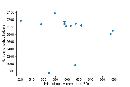
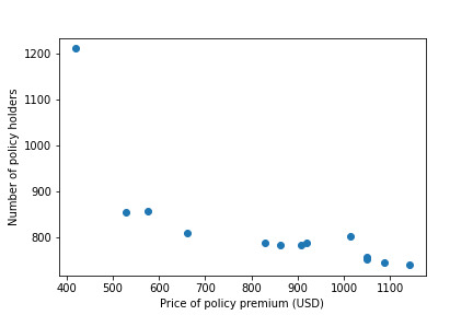
In this work, we model demand sensitivity to insurance premiums through a piecewise linear demand function. We estimate the decline rate using historical data from several states. We include Figures 4 and 5 in the appendix showing the scatterplot of the number of policyholders in a year against the mean policy premium of that state at that year. Different states have different degrees of sensitivity to price, but in general we observe a downward trend of declining policyholder numbers as a function of increased price. For the illustrative purpose of this work, we do not specify different sensitivity in different states but use the same demand-damping function across all states.
We use the following piecewise linear demand-damping function to model demand damping:
f(p)={1,if p≤P0,1−m⋅(p−P0),if p>P0 and f(p)≥cmin,cmin,otherwise.
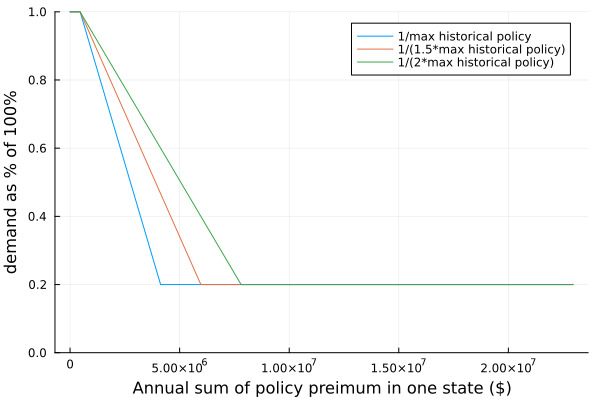
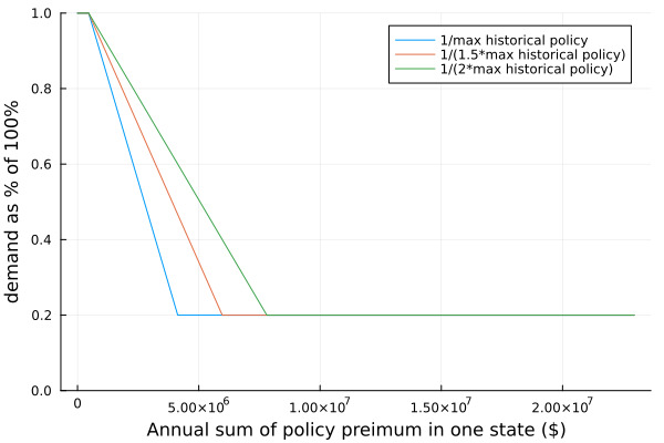
where is the minimum premium at which demand damping starts to occur, and is the minimum fraction of demand. In this work, we choose to be a fraction of maximum historical premium ever charged. We choose to be representing that at least 20% of the total demand is preserved regardless of price. We experimented with different demand-damping rates: We include Figure 6 in the appendix to illustrate several choices of the demand-damping curve.
5. Results
We implement two robust optimization models: RO and ARO. To evaluate their effectiveness, we compare the results against two baseline policy premiums:
-
Historical premiums: The premiums previously charged in each state, referred to as “Hist”.
-
Cumulative moving average (CMA) loss: The average loss up to a given year, denoted as “CMA”. The CMA premium is computed as follows:
pCMAi,t=1tt∑t′=0 li,t′.
A summary of the implemented models is provided in Table 1.
We evaluate performance during the testing period, the last 10 years of available data in the NFIP dataset between 2013 to 2022. For the rest of the section, we choose to be 50,000 and to be 10,000. We also undertake a sensitivity analysis to assess the impact of our model’s parameter selections. Overall, we evaluate our model performance using the following two criteria:
-
Effectiveness: To evaluate the effectiveness of models to cover losses at a state level, we count the number of insolvent states (i.e., the cumulative premium collected over the testing period does not cover cumulative claim losses).
-
Efficiency: To ensure models are charging reasonable levels of premiums to cover losses, we evaluate the overall surplus (or deficit) level as well as the absolute deviation from actual losses to evaluate models’ capabilities in realistically assessing risks.
5.1. Sensitivity analysis
We examine the model’s sensitivity to parameter choices. Specifically, we examine the effect of the value of and the demand-damping rate Recall that is the parameter controlling the conservativeness of the CLT uncertainty set, given by equation (29), and the demand-damping rate controls how fast demand declines in response to increases in price, given by equation (16). To examine the overall performance of the premium, we compute the cumulative surplus across all states over the testing period as follows:
S(γ)=N∑i=1T1∑t=1pi,t−N∑i=1T1∑t=1lhisti,t,
where denotes the historical loss that occurred at location at time
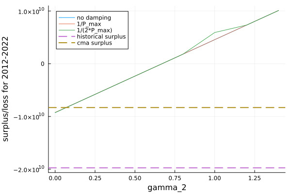
Figure 2 shows the level of surplus as a function of different values, with different demand-damping rates. The two dotted lines show the constant surplus computed by two baselines: using the actual premiums collected during this period and the CMA rule. We observe that both baselines incur a loss over the testing period, with historical premiums resulting in about a $20 billion loss, and the CMA rule resulting in an $8 billion loss.
We let take values between 0 and 1.5 at a step size of 0.1, and we resolve the optimization model at each value and compute the sum of surplus across all states across testing years. corresponds to convex optimization without uncertainty, and corresponds to the maximum degree of uncertainty. As we increase the value of the size of the uncertainty set increases and the model becomes more conservative, resulting in a surplus as expected. We remark that the surplus breaks even when takes a value between 0.6 and 0.7. And we observe a smooth increase in surplus as increases.
In addition, we experiment with three demand-damping rates: no damping, and with damping twice as fast as Similar to as above, we experiment with varying values corresponding to the different demand-damping rates. We observe that the choice of demand damping is less significant compared with the variation of
_computed_for_2012_to_2022_across_all_states_when_varying_the_level_of___.png)
5.2. Effectiveness
Regulators require insurers to protect against insolvency risks, ensuring that premium structures are robust enough to cover potential losses. Therefore, evaluating the effectiveness of insurance schemes in mitigating insolvency is critical. We assess insolvency at the state level, defining a state as insolvent when its cumulative premiums do not cover cumulative losses. This serves as a key indicator of a scheme’s financial resilience and risk management efficiency.
Our analysis spans the 2013–2022 testing period, corresponding to the last 10 years of available data, and focuses on the impact of a parameter that significantly influences model outcomes as indicated in the sensitivity analysis section. As summarized in Table 2, we examine the effects of varying from 0 to 2 in increments of 0.2, evaluating its role in determining the number of insolvent states under each model.
The results in Table 2 highlight substantial differences in the effectiveness of various premium-setting approaches in mitigating insolvency risk. The historical (Hist) scheme performs the worst, resulting in insolvency across all 52 states, underscoring its failure to provide adequate financial protection against catastrophic losses. This outcome reinforces the urgent need for reform in NFIP premium setting in ensuring long-term solvency. The CMA approach, while demonstrating some improvement, still results in insolvency in 36 states. This indicates that although it offers greater stability than the Hist scheme, it lacks the adaptability required to account for evolving risk dynamics. Both the Hist and CMA schemes remain unchanged across different values, as expected.
Both the RO and ARO models demonstrate a clear downward trend in insolvency rates as increases, reflecting their ability to enhance financial resilience through more conservative parameter choices in the uncertainty set. At = 0, these models perform similarly to the CMA approach, with 36 insolvent states, suggesting that without additional conservatism, they do not provide superior risk protection. However, as increases, insolvency rates decline significantly, with ARO consistently outperforming RO across all levels. For instance, at = 1.0, ARO reduces the number of insolvent states to 21, compared to 22 for RO, and at = 2.0, ARO achieves the best performance with just 12 insolvent states, matching the lowest observed insolvency rate. The superior performance of ARO over RO suggests that its adaptive component allows for a more refined approach to premium adjustments under uncertainty. By dynamically incorporating new information, ARO ensures a more robust financial buffer against catastrophic events. The results indicate that higher values lead to more conservative pricing, directly translating into lower insolvency rates. This trade-off underscores the importance of selecting an appropriate value based on risk tolerance and financial strategy. Ultimately, ARO emerges as the most effective method for balancing risk management and capital efficiency, demonstrating its ability to navigate the complexities of catastrophe insurance pricing under uncertainty.
5.3. Efficiency
To evaluate the efficiency of the models, we examine both surplus and deficit levels as well as the absolute deviation (AD) from actual losses. This ensures that models not only mitigate insolvency risks but also avoid excessive overpricing, aligning premiums more accurately with underlying risks.
Table 3 presents the overall surplus (or deficit) levels and AD across all states over the testing period. The AD serves as an indicator of how well each model captures actual risk levels and is computed as a function of as follows:
AD(γ)=N∑i=1T1∑t=1|pi,t−lacti,t|.
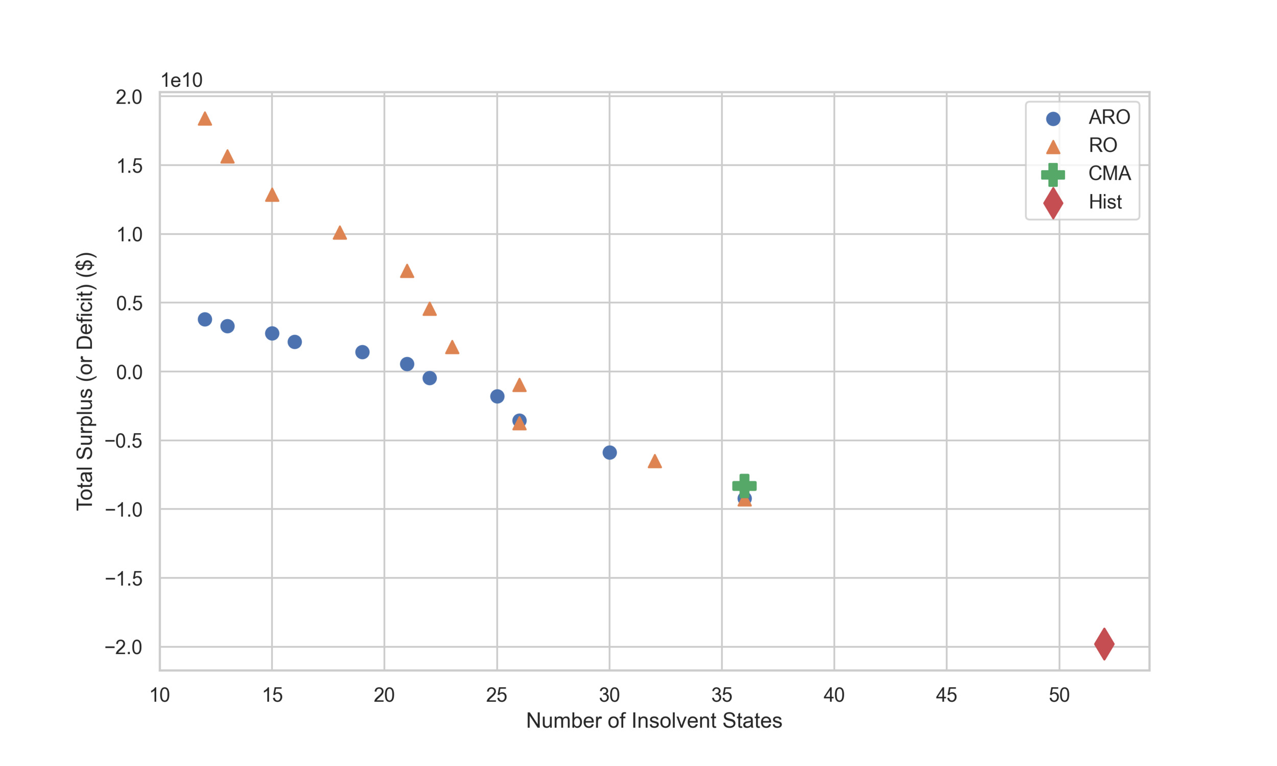
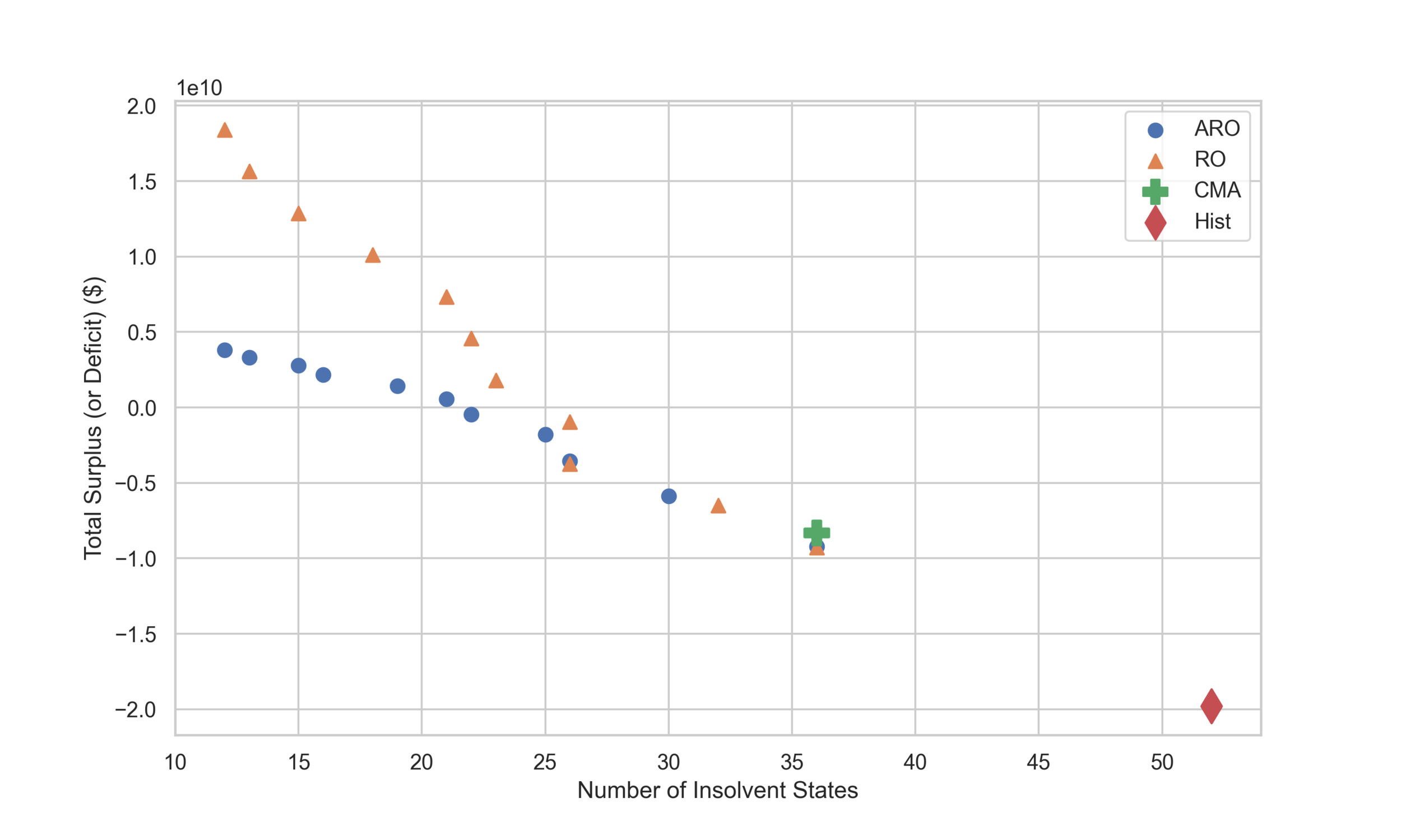
First, we observe that premium setting under the historical scheme significantly undercharges over the testing period, resulting in $19 billion in losses, while the CMA rule results in $8 million in losses. This suggests that historical levels are insufficient to cover future losses. Similar to as before, we observe that as increases, the RO and ARO schemes increase the level of conservatism and achieve more surplus. With the same level of we observe that ARO achieves the surplus more slowly than the RO schemes. Especially when reaches the level of 1.4, the ARO scheme increases premiums much more slowly than the RO schemes, which increases at a constant rate with increasing Figure 3 visualizes the efficient frontier, illustrating the trade-off between the number of insolvent states versus the surplus (or deficit) achieved during the testing period.
Both the RO and ARO models exhibit a clear trend of increasing surplus as rises, demonstrating their ability to enhance financial resilience by incorporating greater conservatism in pricing. At RO and ARO perform similarly to CMA, both exhibiting a deficit of approximately $9.2 billion, indicating that without additional conservatism, these models do not provide better financial protection. However, as increases, ARO and RO gradually transition from a deficit to surplus. For instance, at the ARO scheme achieves a surplus of $0.55 billion, while RO reaches $4.57 billion. At the highest level, RO achieves a surplus of $18.41 billion, compared to $3.82 billion for ARO. RO accumulates surplus at a significantly higher rate than ARO, suggesting that ARO adjusts premiums more gradually, while RO adopts a more aggressive pricing strategy. This difference arises because ARO premiums are influenced by the previous year’s losses, thus allowing for greater flexibility and a more measured response to risk fluctuations. A key distinction between ARO and RO emerges as increases, particularly at where RO reaches a $10.11 billion surplus, while ARO remains at $2.16 billion. This suggests that ARO incorporates uncertainty more dynamically, whereas RO increases premiums at a near-linear rate with This controlled adjustment process in ARO makes it preferable for policymakers seeking a stable and adaptable pricing framework. In contrast, RO provides a more aggressive pricing approach, accumulating a higher surplus but at the cost of higher absolute deviation, which may indicate overpricing.
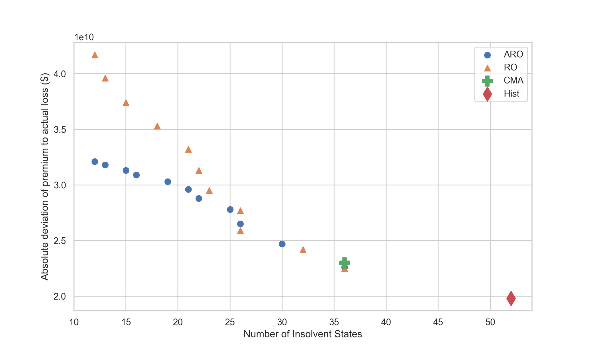
The AD metric provides insights into how well each model aligns premiums with actual incurred losses. The historical scheme has the lowest AD but that is due to severe underpricing rather than accurate risk estimation, as evidenced by its extreme deficit. The CMA scheme maintains an AD of Both the RO and ARO schemes lead to an increase in AD as increases, while they become more conservative. They also tend to deviate more from actual losses. However, ARO consistently maintains a lower AD than RO, highlighting that ARO balances conservatism with pricing accuracy more effectively.
The trade-off between insolvency risk and surplus generation is further illustrated in Figure 3, which depicts the number of insolvent states against the surplus/deficit levels. The results indicate that while increasing improves financial resilience, it also leads to higher absolute deviation from actual losses. ARO emerges as the most balanced scheme, providing strong insolvency protection while avoiding excessive overpricing. RO, on the other hand, is better suited for highly risk-averse insurers who prioritize surplus accumulation over pricing efficiency. The Hist and CMA schemes fail to provide sustainable financial protection, reinforcing the necessity of adopting dynamic, uncertainty-aware premium-setting strategies.
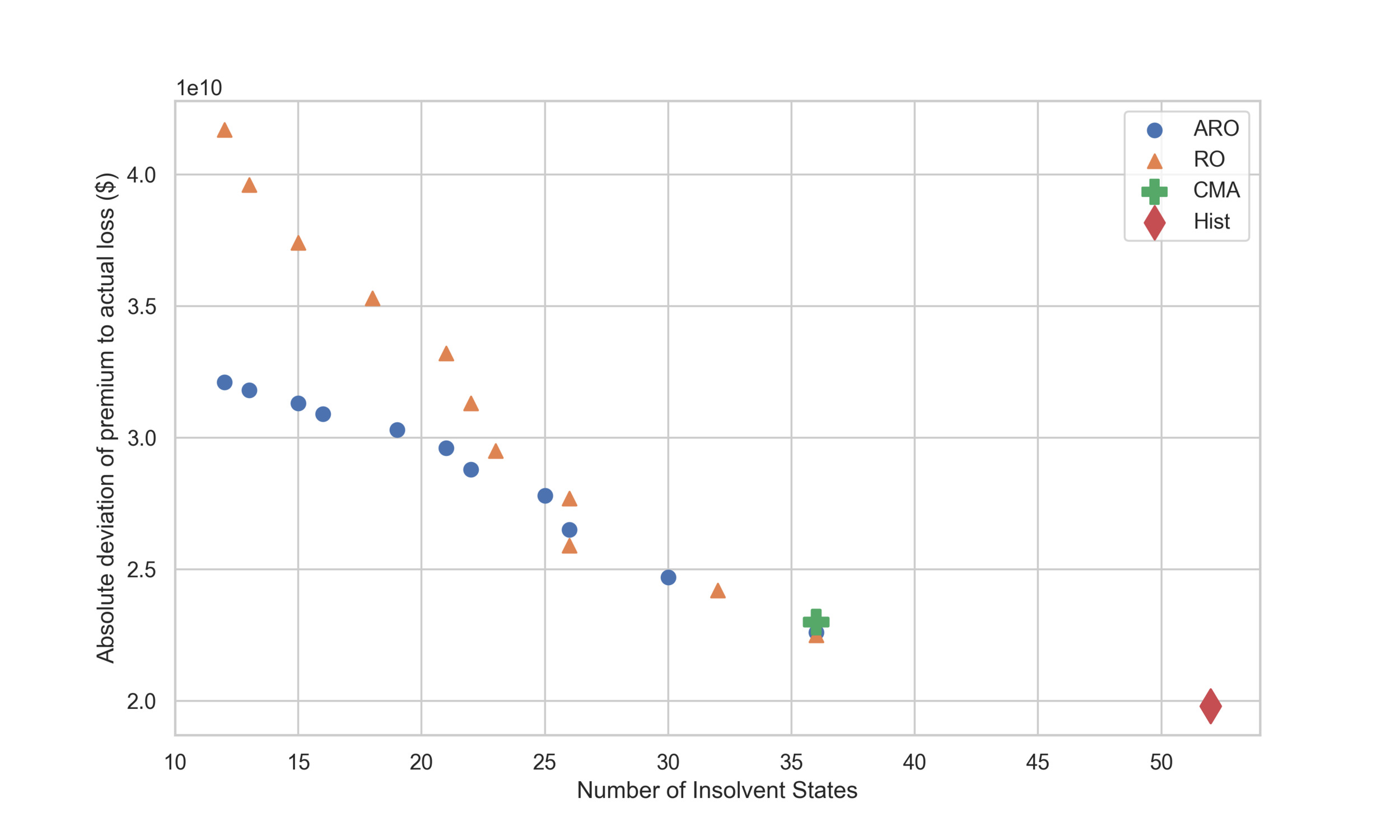
In conclusion, the results confirm that ARO is the most effective model for balancing financial stability, premium efficiency, and risk alignment. Although RO achieves the highest surplus, it does so at the cost of higher deviation, making it more suitable for risk-averse regulators. In contrast, ARO provides a more stable pricing strategy with controlled surplus accumulation, making it a more pragmatic choice for long-term catastrophe insurance pricing. Figure 7, included in the appendix, further explores the trade-off between the number of insolvent states and absolute deviation during the testing period.
6. Conclusion
In this work, we present an ARO framework for catastrophe insurance premium pricing, designed to balance insolvency risk and capital efficiency. We first introduce a nominal linear optimization formulation to frame the challenge of setting insurance prices for rare catastrophic events. We then extend this to an RO model incorporating a central limit theorem uncertainty set, ensuring protection against volatility in losses modeled from historical distributions. By solving the inner problem in closed form, we derive the robust counterpart and reformulate it as a convex optimization problem. Further, we develop an ARO model using linear decision rules allowing for dynamic premium adjustments based on actual loss experiences, improving responsiveness to evolving risk conditions.
We apply our ARO framework to the realm of US flood insurance, leveraging data from the NFIP. We evaluate performance against two benchmark schemes—NFIP premiums and CMA premiums. Historical data from 1975 to 2012 were used to construct uncertainty sets, and the last 10 years of NFIP data were used to assess out-of-sample performance. Our results demonstrate that optimization-based approaches effectively cover losses at the same time as they provide flexibility to policymakers in adjusting premiums based on risk tolerance and degree of conservatism.
Our findings point to two key advantages of the ARO framework:
-
Effectiveness: The ARO approach significantly reduces insolvency risk by effecting a smooth transition from a high number of insolvent states to a low and controllable level as conservatism increases. Unlike static benchmarks, which fail to adapt to risk variations, the ARO scheme provides policy providers with flexibility to determine the desired insolvency level while maintaining financial stability.
-
Efficiency: The ARO scheme efficiently adjusts premiums to strike a balance between financial sustainability and affordability. Unlike RO, which aggressively increases surplus at increasingly conservative levels, ARO maintains a more controlled surplus accumulation, avoiding excessive overpricing. The model enables a smooth transition from deficit to surplus, ensuring that insurers are neither overexposed to risk nor excessively charging policyholders.
The ARO framework is adaptable and generalizable to a broad class of catastrophic events beyond floods, including wildfire, drought, and extreme weather events. ARO’s flexibility makes it a promising tool for insurers and policymakers who wish to develop sustainable, data-driven pricing strategies for managing climate- and disaster-related risks.
.png)
.png)