Sensitivity of Complex Reinsurance Pricing Metrics to Model Assumptions

1. Introduction

The earth’s climate system gives rise to events such as hurricanes, mid-latitude windstorms, wildfires, and severe convective storms. The insurance industry creates value by enabling transfer of risk arising from such events. For example, homeowners pay annual premiums to insurers for the right to claim recoveries after damaging events. Insurers purchase reinsurance to diversify risk and improve profitability. Pricing of reinsurance contracts is dependent on economic factors, market dynamics, and technical metrics derived from risk models. This paper focuses on technical pricing metrics from the point of view of the reinsurer.

The motivation behind this paper was to increase understanding of how climate change and reinsurance pricing may interact. A major premise of climate change science is that human-induced increases in greenhouse gas concentrations, such as carbon dioxide and methane, have a direct causal link to large-scale changes in the earth’s climate system. This claim is supported by the peer-reviewed scientific literature (see Lynas et al. 2021, which describes the authors’ analysis of 88,125 climate-related papers written between 2012 and 2020). Climate change has recently been front and center in the insurance industry, which is clear from articles written by a spectrum of stakeholders, including rating agencies and analytics firms (Moody’s 2024), reinsurance brokers (WTW 2024), regulatory bodies (Hielkema 2023), consulting firms (Fantini et al. 2023), accounting firms (PWC 2024), actuarial organizations (Climate Change Working Party 2020), reinsurers (Zaitsev 2021), and popular science publications (Frank and E&E News 2023).

The idea that climate change impacts the frequency and severity of natural catastrophes also has scientific consensus (Seneviratne et al. 2021; Calvin et al. 2023)—suggesting that natural catastrophe risk models that fail to account for climate change must be “perturbed” in some fashion, raising questions, such as: What impact do these model perturbations have on reinsurance pricing metrics? What fundamental understanding and/or framework can reinsurers use to handle perturbed risk profiles arising from climate change? This is a complex and important problem that few studies have investigated (e.g., Khare 2024; Khare and Roy 2021; note that we use the notation provided in Khare 2024). To advance understanding in this area, we used a top-down approach that represents the natural catastrophe risk model setup using a simplified frequency and severity model appropriate to a US-wide industry portfolio covering four climate perils (hurricane, windstorm, wildfire, and severe convective storm). The risk model employed here is the same as that in Khare and Roy (2021), with the earthquake peril excluded. Anecdotally, we note that private sector catastrophe risk models used in practice are based on complex bottom-up models using cutting-edge climate science, engineering, financial concepts, and large-scale cloud computing (see Golnaraghi et al. 2018 for a discussion of these topics). Our simplified top-down approach allows us to run a comprehensive sensitivity analysis enabling fundamental insights (traded for a degree of realism).

Using a representative US nationwide portfolio, this paper makes the following contributions:

• Explores the sensitivity of reinsurance price metrics to model parameter perturbations and contract assumptions for a wide range of catastrophe excess of loss (catXL) layers

• Presents a framework for how reinsurers can consider strategy when dealing with model perturbations

• Clarifies various trade-offs made by reinsurers when increasing/decreasing the risk profile of underwritten reinsurance layers

• Provides insights into how reinsurers can manage climate change from a technical perspective

• Presents a framework for understanding the implications of recent property catastrophe market dynamics (as of 2024)

We emphasize that our work is applicable to reinsurers whose portfolios are well approximated by proportional slices of the US nationwide industry portfolio; to some degree this limits the generalizability of this work. However, the method of analysis and framework presented in this paper can be applied to more general cases, as will be discussed. The paper is formatted as follows: Section 2 reviews mathematical definitions and assumptions, provides details on the base (unperturbed) natural catastrophe model, and discusses both analytical and numerical approaches to formulating catastrophe excess of loss (catXL) reinsurance pricing metrics. Section 3 briefly discusses the risk profile of the base natural catastrophe model, describes our numerical experiments and numerical accuracy, presents core results, and ends by discussing the fundamental insights derived from our results. Section 4 provides a summary, discusses the implications of our work for reinsurer strategy under climate change, sheds light on recent market dynamics, and discusses future research directions. Appendices A, B, and C provide mathematical details that underpin the analytical and numerical methods we employed.

2. Preliminaries

This section discusses various mathematical definitions and assumptions, the multiperil frequency and severity model used as our base natural catastrophe model, analytical formulations for the catXL reinsurance contract central to this work, and various numerical schemes we employed to compute contract pricing metrics.

2.1. Mathematical definitions and assumptions

The following provides elementary definitions for completeness and begins by defining the frequency component of our representative natural catastrophe model.

Definition 2.1. Frequency distribution: The random number of events over a specified time interval (one year in this work) is denoted by $N$ and has a discrete frequency distribution $P_{N}(k)$, where $k\in[0,1,2,..,\infty)$, and $\sum_{k=0}^{\infty}P_{N}(k)=1$.

In this work all frequency distributions are Poisson, which is defined as follows.

Definition 2.2. Poisson frequency distribution: The Poisson frequency is

$$P_{N}(k)=\frac{e^{-\lambda}\lambda^{k}}{k!},$$

where the expectation $\mathbb{E}\left[N\right]=\lambda$ is a positive real number representing the annual average rate of events and the variance $\mathbb{V}\left[N\right]=\mathbb{E}\left[N\right]$.

For a given event occurrence, the random financial loss $X$ (for a particular portfolio of physical assets) is drawn from a severity distribution defined as follows.

Definition 2.3. Severity distribution: The continuous severity density is

$$f_{X}(x),$$

where $x\in[0,\infty)$ (and $\int_{0}^{\infty}f_{X}(x)dx=1$).

Individual peril severities are modeled using continuous gamma distributions defined as follows.

Definition 2.4. Gamma distribution: The gamma distribution is

$$g_{X}(x)=\frac{x^{\alpha-1}e^{-\beta x}}{\Gamma(\alpha)\beta^{-\alpha}},$$

where $x\in(0,\infty)$, the shape parameter $\alpha>0$, the scale parameter $\beta>0$, and $\mathbb{E}\left[X\right]=\alpha\beta$ and $\mathbb{V}\left[X\right]=\alpha\beta^{2}$.

For simplicity we impose the assumption that samples from $P_{N}(k)$ and $f_{X}(x)$ are drawn independently (this is common in many applications, see Shi et al. 2015 for generalizations). The combination of the frequency $P_{N}(k)$ and severity $f_{X}(x)$ represents a mathematical abstraction of a risk model applied to a specific portfolio of assets. Our top-down approach allows us to rapidly explore the effects of alternative model assumptions, which is the central focus of this work.

Timeline simulation is a central concept in risk modeling, so reviewing the concept is helpful for setting up the reinsurance pricing problem. It involves sampling both $P_{N}(k)$ and $f_{X}(x)$ in a sequence that generates losses for a specified set of simulation years and is defined as follows.

Definition 2.5. Timeline simulation: A timeline simulation for $S$ years is defined by the following process:

1. For all years indexed by $i=1,...,S$,

2. Draw a random number from the frequency distribution $P_{N}(k)$,

3. For each year $i$ let the random realization be $N=k_{i}$, which implies that we must take $k_{i}$ random (loss) samples from the severity $f_{X}(x)$ (all samples are tagged with year $i$).

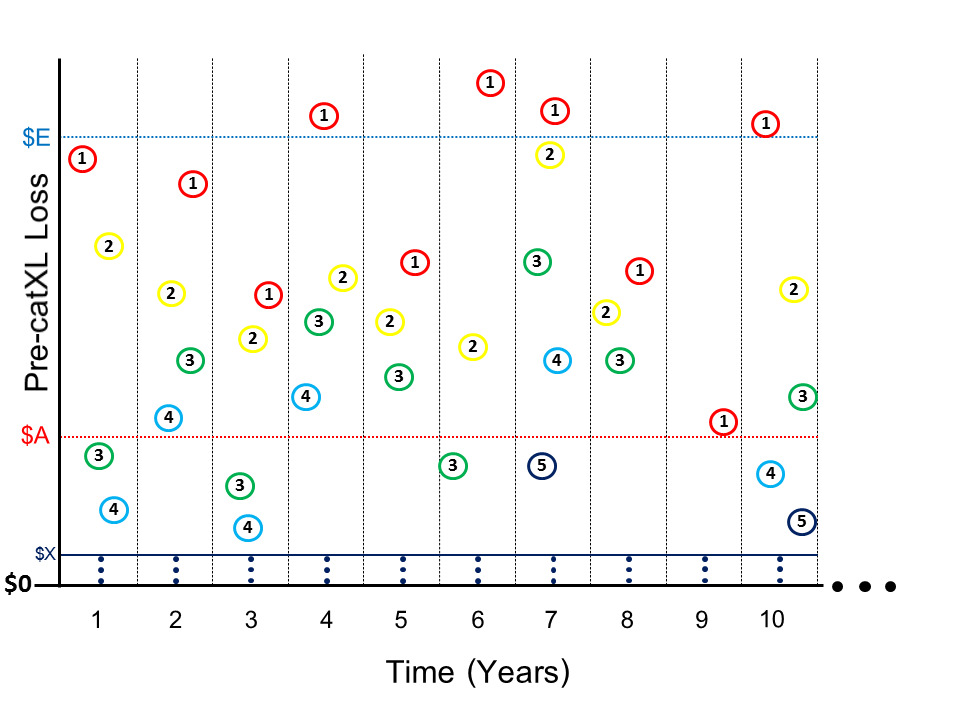
For clarification, see the visualization in Figure 1.

Figure 1.Sensitivity of reinsurance pricing metrics. The figure depicts a timeline simulation for a given frequency $P_N(k)$ and severity $f_X(x)$. Each simulation period is one year in length (x-axis), and the y-axis shows the primary insurer portfolio loss in dollars before any reinsurance is applied. The annual maximum loss events are depicted by the 1s with red circles; the second annual maximum losses are indicated by the 2s with yellow circles, and so on. Event losses that are less than or equal to $X < $A have values in the closed interval from $0 to $X. The dashed red and blue lines indicated by the $A and $E values correspond to the attachment and exhaustion point of a catXL reinsurance contract that will be applied in what follows. Events with losses below $X are not depicted.

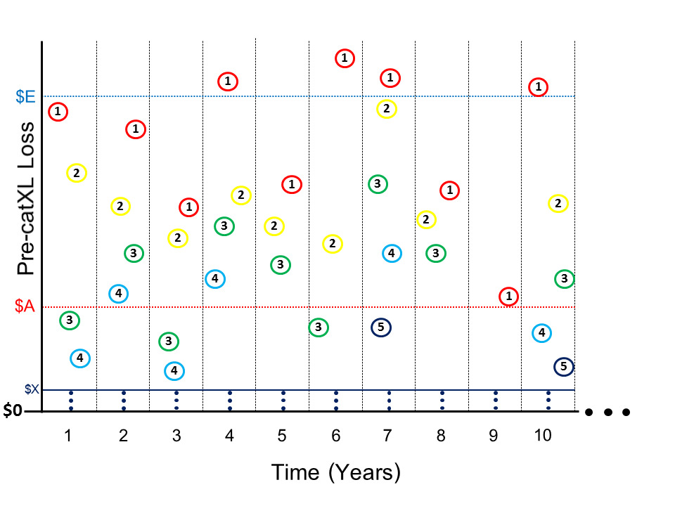
Figure 1 depicts a timeline simulation generated from a given $P_{N}(k)$ and $f_{X}(x)$. The y-axis represents loss to a primary insurer before the application of reinsurance; “pre-catXL” on the y-axis makes clear the losses are depicted before applying a catXL contract. The catXL contract is represented by the attachment point $A and exhaustion point $E. Losses within the layer (up to a prespecified annual limit) are the responsibility of the reinsurer. Figure 1 also explicitly denotes the order statistics (Barakat and El-Shandidy 2004; Buhrman 1973; Consul 1984; David and Nagaraja 2003; Gupta and Gupta 1984; Young 1970; Khare 2024; Khare and Roy 2021). The red circled 1s depict the annual maxima, the yellow circled 2s the second annual maxima, and so on. In practical applications the order statistics are typically referred to as occurrence losses. We now discuss our parameterization of $P_{N}(k)$ and $f_{X}(x)$ for the base natural catastrophe model, followed by a discussion of technical catXL pricing metrics.

2.2. Multiperil base climate natural catastrophe model for a US nationwide portfolio

Our overarching aim is to shed light on the impact of model uncertainty (arising from sources such as climate change) in reinsurance pricing using a representative multiperil base natural catastrophe model. Several factors were considered in formulating the base model:

• Maintaining consistency with previously published actuarial and risk literature

• Deriving model parameter settings from publicly available information

• Using commonly applied frequency and severity distributions

• Providing a straightforward way to perform sensitivity analysis (relevant to climate change/variability)

• Representing a large industry level portfolio in a major reinsurance market like the United States

The model setup employed in Khare and Roy (2021) meets these various considerations. The authors used publicly available information to parameterize the frequency and severity of several perils applicable to a large US nationwide portfolio of insured assets (see Khare and Roy 2021 for detailed justification). The model consists of four climate perils: hurricane (HU), winter storm (WS), wildfire (WF), and severe convective storm (SCS). The base model parameters are extracted from Khare and Roy (2021, Table 1) and repeated here in Table 1.

The parameters in Table 1 represent a range of important perils comprising both high frequency, low severity perils (SCS with $\mathbb{E}\left[N_{SCS}\right]=100$, where $N_{SCS}$ denotes the discrete random variable) and low frequency, high severity perils (HU with $\mathbb{E}\left[N_{HU}\right]=2$). WF is high frequency but has much higher severity volatility ($CV=8$) compared with SCS ($CV=4$), consistent with the nature of the perils. The multiperil climate natural catastrophe model is formulated as a mixture. For the frequency distribution, as each individual peril is Poisson and independent of all other perils, the multiperil frequency random variable is taken to be $N=N_{HU}+N_{WS}+N_{W}+N_{SCS}$, and is Poisson distributed with $\scriptsize \lambda=\mathbb{E}\left[N\right]=\mathbb{E}\left[N_{HU}\right]+\mathbb{E}\left[N_{WS}\right]+\mathbb{E}\left[N_{WF}\right]+\mathbb{E}\left[N_{SCS}\right]=178$ (e.g., Krishnamoorthy 2015). The severity distribution for each peril is gamma distributed. A unique set of $\alpha$ and $\beta$ parameters are chosen for each peril given the target average annual loss (AAL), expected frequency, and severity distribution coefficient of variation (CV), where $CV=\frac{\sqrt{\mathbb{V}\left[X\right]}}{\mathbb{E}\left[X\right]}$. For example, the expectation of the severity for HU is equal to $12.5 billion divided by 2 ($\mathbb{E}_{HU}\left[N\right]=2$), which is $6.25 billion; combined with the target $CV$ of 5 we can infer the $\alpha$ and $\beta$ parameters listed in the table. The multiperil severity distribution $f_{X}(x)$ is formulated as a mixture model where the weights are in proportion to the rates given by

$$\begin{align} f_{X}(x)&=w_{HU}f_{HU,X}(x)+w_{WS}f_{WS,X}(x) \\&\quad+w_{WF}f_{WF,X}(x)+w_{SCS}f_{SCS,X}(x), \end{align}$$

with $w_{HU}=\frac{\mathbb{E}\left[N_{HU}\right]}{\mathbb{E}\left[N\right]}$, $w_{WS}=\frac{\mathbb{E}\left[N_{WS}\right]}{\mathbb{E}\left[N\right]}$, $w_{WF}=\frac{\mathbb{E}\left[N_{WF}\right]}{\mathbb{E}\left[N\right]},$ and $w_{SCS}=\frac{\mathbb{E}\left[N_{SCS}\right]}{\mathbb{E}\left[N\right]}$ (note that $w_{HU}+w_{WS}+w_{WF}+w_{SCS}=1$, and $\int_{0}^{\infty}f_{X}(x)=1$), and $f_{HU,X}(x)$ is the hurricane-specific severity (which is similarly depicted in other perils). As stated above, the multiperil frequency and severity distributions are sampled independently.

2.3. Analytical formulations of catXL pricing metrics

This work studies the catXL contract with reinstatements (Mata 2000; Cummins et al. 1999), providing analysis of loss metrics from the point of view of the reinsurer. For a catXL contract, the reinsurer is responsible for the payout of all event losses, as shown in Figure 1, beginning just above the attachment point $$A$ up to an event maximum of $$(E-A)$, subject to an annual aggregate limit $A_{lim}=(n+1)(E-A)$, where the integer $n\geq0$. Note that $n$ is called the number of reinstatements because it represents a multiplier on the “width of the layer” given by $$(E-A)$. To proceed we must define an annual aggregate loss random variable that depends on the contract parameters $$A$, $$E, A_{lim}.$ As in Khare and Roy (2021), the mean and standard deviation of this annual aggregate loss random variable will be used to compute a “technical price,” which is the focus of this work. We start by defining the annual aggregate loss random variable $Y$ prior to the application of any reinsurance (pre-catXL). Using classical compound notation (Klugman et al. 2008) we have the following definition.

Definition 2.6. Pre-catXL annual aggregate loss random variable: The annual aggregate loss is

$$Y=X_{1}+...+X_{N},$$

where $X_{i}\thicksim f_{X}(x)$ for all $i=1,...,N,$ and the number of events is random where $N\thicksim P_{N}(k).$

We now define the annual aggregate loss random variable for the reinsurer. First, for a given layer defined by attachment point $$A$ and exhaustion $$E$, we must apply an operator to all samples of $f_{X}(x).$ This operator results in a transformed random variable: $X_{AE}\equiv min\left[max\left[0,X-A\right],E-A\right]$ (all losses below attachment $$A$ are set to zero, the payout is $X-A$ up to the maximum $E-A$). We call $X_{AE}$ the “post-catXL” severity random variable. With $X_{AE}$ in hand, we are ready to define the post-catXL annual aggregate loss random variable.

Definition 2.7. Post-catXL annual aggregate loss random variable: The annual aggregate loss is

$$Y_{AE}=min\left[X_{1,AE}+...+X_{N,AE},A_{lim}(n)\right],$$

where $X_{i,AE}=min\left[max\left[0,X_{i}-A\right],E-A\right]$ where $X_{i}\thicksim f_{X}(x)$ for $i=1,...,N$, $A_{lim}(n)=(n+1)(E-A)$ with reinstatements $n\in[0,1,2,...,\infty)$, and the random number of events $N\thicksim P_{N}(k).$

We emphasize that $Y_{AE}$ is defined for a particular fixed aggregate limit $A_{lim}$ for a specified number of reinstatements $n$ (not made explicit in our notation to keep it succinct). Reinsurers can use the distribution of $Y_{AE}$ to quantify technical metrics that aid in the underwriting and portfolio management. Here we study the expectation $\mathbb{E}\left[Y_{AE}\right]$ and standard deviation $\mathbb{S}\left[Y_{AE}\right]$ (and their sum). This is motivated by common market practice where a technical pricing metric $T$ is used, and is formulated as

$$T=\frac{\mathbb{E}\left[Y_{AE}\right]+\nu\mathbb{S}\left[Y_{AE}\right]}{P_{net}},$$

where $\nu$ is a volatility “loading factor,” and $P_{net}$ is the net premium, which the reinsurer receives as compensation for taking responsibility for the losses $Y_{AE}$ (Khare and Roy 2021). Other factors, such as diversification debit or credit in the context of the entire reinsurer portfolio, are typically considered in practice but are outside the scope of this work. The aim of this paper is to understand the effect of model parameter changes (around the base model specified in Section 2.2) on the metrics $\mathbb{E}\left[Y_{AE}\right]$ and $\mathbf{\mathbb{S}}\left[Y_{AE}\right]$ and their sum $\mathbb{E}\left[Y_{AE}\right]+\mathbb{S}\left[Y_{AE}\right]$ for a variety of practically relevant contract setups.

To simplify the complex sensitivity analysis to follow, we have not included an aggregate deductible in defining $Y_{AE}$ as was done in previous work (Hürlimann 2005; Mata 2000). Our notation is designed to be consistent with the recent paper on catXL pricing that motivated this work, Khare and Roy (2021).

2.4. Computational methods for computing catXL pricing metrics

Our objective is to compute the pricing metrics $\mathbb{E}\left[Y_{AE}\right]$ and $\mathbb{S}\left[Y_{AE}\right]$ for a given attachment $$A$, exhaustion $$E,$ and specified number of reinstatements $n$, with aggregate limit $A_{lim}=(n+1)(E-A).$ All the main sensitivity results for any $n\geq0$ presented in this work compute $\mathbb{E}\left[Y_{AE}\right]$ and $\mathbb{S}\left[Y_{AE}\right]$ using the fast Fourier transform (FFT) method discussed in Appendix C. We believe other methods could be employed to compute $\mathbb{E}\left[Y_{AE}\right]$ and $\mathbb{S}\left[Y_{AE}\right]$, but we used the FFT method because it was found to be suitable for our application. To increase confidence in our results and implementation, we also conducted various accuracy tests, which are discussed in what follows.

2.4.1. Accuracy check on FFT implementation for computing $\mathbb{E}\left[Y_{AE}\right]$ and $\mathbb{S}\left[Y_{AE}\right]$

To gauge the numerical accuracy of our FFT implementation, we can compare $\mathbb{E}\left[Y_{AE}\right]$ and $\mathbb{S}\left[Y_{AE}\right]$ computed using our FFT method with results derived from numerical integration, specifically for the case where $n\rightarrow\infty.$ The numerical integral method to obtain $\mathbb{E}\left[Y_{AE}\right]$ and $\mathbb{S}\left[Y_{AE}\right]$ in the $n\rightarrow\infty$ limit is discussed in Appendix B. The integral formulas are solved using numerical methods found in the NumpPy Python libraries (Harris, Millman, and van der Walt 2020). We assumed that if the FFT method compares well with the results derived from numerical integration for the $n\rightarrow\infty$ case, it is accurate for all cases. The justification for this is discussed in Appendix C.

2.4.2. Technical pricing metrics using discrete Fourier transforms: all cases ($n \geq 0$)

Appendix C reviews the details behind our FFT based calculations of $\mathbb{E}\left[Y_{AE}\right]$ and $\mathbb{S}\left[Y_{AE}\right]$. A few necessary details are provided here to make our implementation clear. The main idea is to compute a discrete vector of probabilities that accurately represents the post-catXL aggregate loss distribution for any $$A$, $$E$, and $n$. This is readily used to compute $\mathbb{E}\left[Y_{AE}\right]$ and $\mathbb{S}\left[Y_{AE}\right]$.

A numerical grid is formed as $x_{[0]},x_{[1]},...,x_{[M-1]}$, where $x_{[0]}=0$ and $x_{[M-1]}=L_{max}-A$, $L_{max}$ is a fixed “maximum loss,” and $M$ is the number of grid points. The grid spacing is constant for a given catXL layer with $\triangle x=x_{i+1}-x_{i}=\frac{L_{max}-A}{M}$ for $i=0,...,M-2$. Appendix C formulates the probability vector ${\bf p}_{S,AE,n}$, which is the $M-$dimensional vector where ${\bf p}_{S,AE,n,[i]}$ is the probability of the annual loss $Y_{AE}$ we assign to each discrete grid point from $i=0$ to $i=M-1$ for a given $n$ and $A_{lim}=(n+1)(E-A)$.

From ${\bf p}_{S,AE,n}$, we then apply standard formulas to compute the technical pricing metrics as

$$\mathbb{E}\left[Y_{AE}\right]=\sum_{i=0}^{M-2}{\bf p}_{S,AE,n,[i]}x_{i},$$

and

$$\mathbb{S}\left[Y_{AE}\right]=\sqrt{\sum_{i=0}^{M-2}\frac{{\bf p}_{S,AE,n,[i]}\left(x_{[i]}-\mathbb{E}\left[Y_{AE}\right]\right)^{2}}{M-1}}.$$

We emphasize that the above is applicable to all cases for any combination of $n$, $$A$, $$E$ including the pre-catXL case (if $$A=0$, $$E\rightarrow\infty$ and $n\rightarrow\infty$). The accuracy of the probabilities (and in turn $\mathbb{E}\left[Y_{AE}\right]$ and $\mathbb{S}\left[Y_{AE}\right]$) is contingent on the number of grid points $M,$ and the choice of the maximum modeled loss $L_{max}.$ We used fixed values for $M$ and $L_{max}$, which are chosen to achieve accurate results across the entire set of reinsurance layers and model configurations examined in this work (numerical accuracy results are discussed in Section 3). We use fast FFT methods where $M$ is chosen as a power of $2$ (to optimize computational speed), and $L_{max}$ is large enough to provide an appropriate degree of “zero padding” required for accuracy. See Brigham (1988) for a complete discussion of discrete Fourier transform methods.

2.4.3. Measuring numerical accuracy of FFT based aggregate loss metrics

The accuracy of the FFT implementation is dependent on our choices for the maximum modeled loss $L_{max}$ and grid size $M.$ We now detail our method for comparing FFT and numerical integral results for the $n\rightarrow\infty$ case. As discussed above, we assume that if accurate results are obtained when $n\rightarrow\infty$, the FFT method is accurate for all cases. Our rationale is provided in Appendix C. The integral results for a given catXL layer are denoted $\mathbb{E}^{I}\left[Y_{AE}\right]$ and $\mathbb{S}^{I}\left[Y_{AE}\right]$, respectively (where we use superscript $I$ to indicate integration). The analogous results for the FFT method are denoted $\mathbb{E}^{F}\left[Y_{AE}\right]$ and $\mathbb{S}^{F}\left[Y_{AE}\right]$ (for a given $A$, $E$, $L_{max}$, $M$, and $n\rightarrow\infty$). We use two methods to quantify accuracy: (1) absolute percentage errors to the targets $\mathbb{E}^{I}\left[Y_{AE}\right]$ and $\mathbb{S}^{I}\left[Y_{AE}\right]$ and (2) the “effective number of years of simulation” using standard errors (Wasserman 2004). Clearly $\mathbb{E}^{F}\left[Y_{AE}\right]$ is not a random variable estimated from independent and identically distributed samples from a well-defined distribution, but for the sake of assessing accuracy, we treat it as though it were, and make use of the central limit theorem (Wasserman 2004) to characterize the absolute error as

$$abs\left(\mathbb{E}^{F}\left[Y_{AE}\right]-\mathbb{E}^{I}\left[Y_{AE}\right]\right)=\frac{\mathbb{S}^{I}\left[Y_{AE}\right]}{\sqrt{S_{eq}}},$$

where $\mathbb{E}^{I}\left[Y_{AE}\right]$ and $\mathbb{S}^{I}\left[Y_{AE}\right]$ are deemed as the true values, $\mathbb{E}^{F}\left[Y_{AE}\right]$ is the FFT result (dependent on the numerical setup including $M$, the number of grid points), and $S_{eq}$ is what we call the “equivalent number of simulation years” analogous to the number of independent and identically distributed samples. Clearly,

$$S_{eq}=\left(\frac{\mathbb{S}^{I}\left[Y_{AE}\right]}{abs\left(\mathbb{E}^{F}\left[Y_{AE}\right]-\mathbb{E}^{I}\left[Y_{AE}\right]\right)}\right)^{2}$$

serves as a useful alternative measure of accuracy, since the number of years terminology is commonplace in applied risk modeling (Definition 2.5). The above formulation is used for the pre-catXL case where $Y_{AE}$ is replaced by $Y.$

3. Numerical experiments and discussion

Sections 3.1, 3.2, and 3.3, respectively, cover the base model loss profile, the design of our numerical experiments, and details on the numerical accuracy of our FFT calculations, which sets the stage for the core numerical results presented in Sections 3.4, 3.5, and 3.6. Section 3.4 presents numerical results for two extreme cases made up of a low and high catXL layer. Section 3.5 discusses intermediate cases lying between our low and high layers. Section 3.6 reviews key findings and insights garnered from our numerical work.

3.1. Base model loss distribution profile

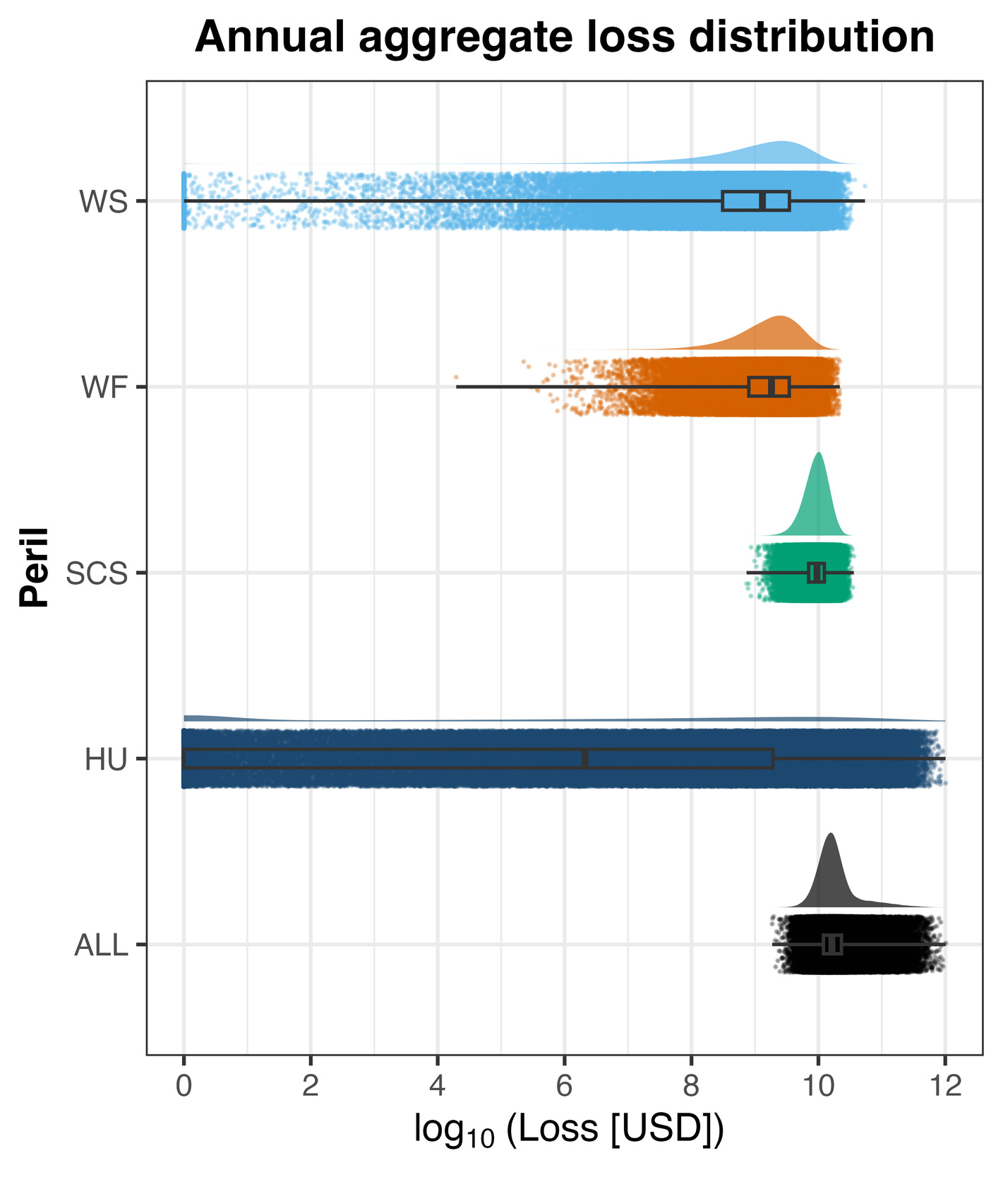
Figure 2 displays results from a $S=500K$ year timeline simulation for the base model (Section 2.2). Annual aggregate losses are displayed for the four perils (WS, WF, SCS, and HU), including a histogram and bars that indicate the min, max, and interquartile ranges (losses are spread vertically for display purposes only). Figure 2 reveals interesting differences in the annual aggregate losses across the perils. For example, the HU losses are highly volatile and reach far into the tail (with the highest loss of order $10^{12}$). SCS annual aggregate losses are much higher than those of WF and WS but also much less volatile, reflecting its high frequency and low volatility (compared with WF). The full group of multiperil losses are labeled “ALL” and depicted in the final set of results in Figure 2. The content in Figure 2 suggests that the contributions of the perils will depend on the particular catXL contract in question (with parameters $$A,$ $$E$, and $n$). Figure 2 makes clear the materiality of the annual losses for the case studied in this work with significant probability above US$$100$ billion.

Figure 2.Annual aggregate loss distribution. This figure displays results from a $\mathrm{S}=500 \mathrm{~K}$ year timeline simulation derived from the multiperil frequency and severity model, which shows the annual aggregate losses for winter storm (WS), wildfire (WF), severe convective storm (SCS), and hurricane (HU). The colored dots represent the annual aggregate losses overlaid by a bar indicating the minimum, maximum, median, and interquartile ranges. A histogram is also provided for each peril. The final set of results (labeled ALL) displays the analogous results for the four perils aggregated. Note that this figure is identical to Figure 3 of Khare and Roy (2021), except for earthquake, which is excluded.

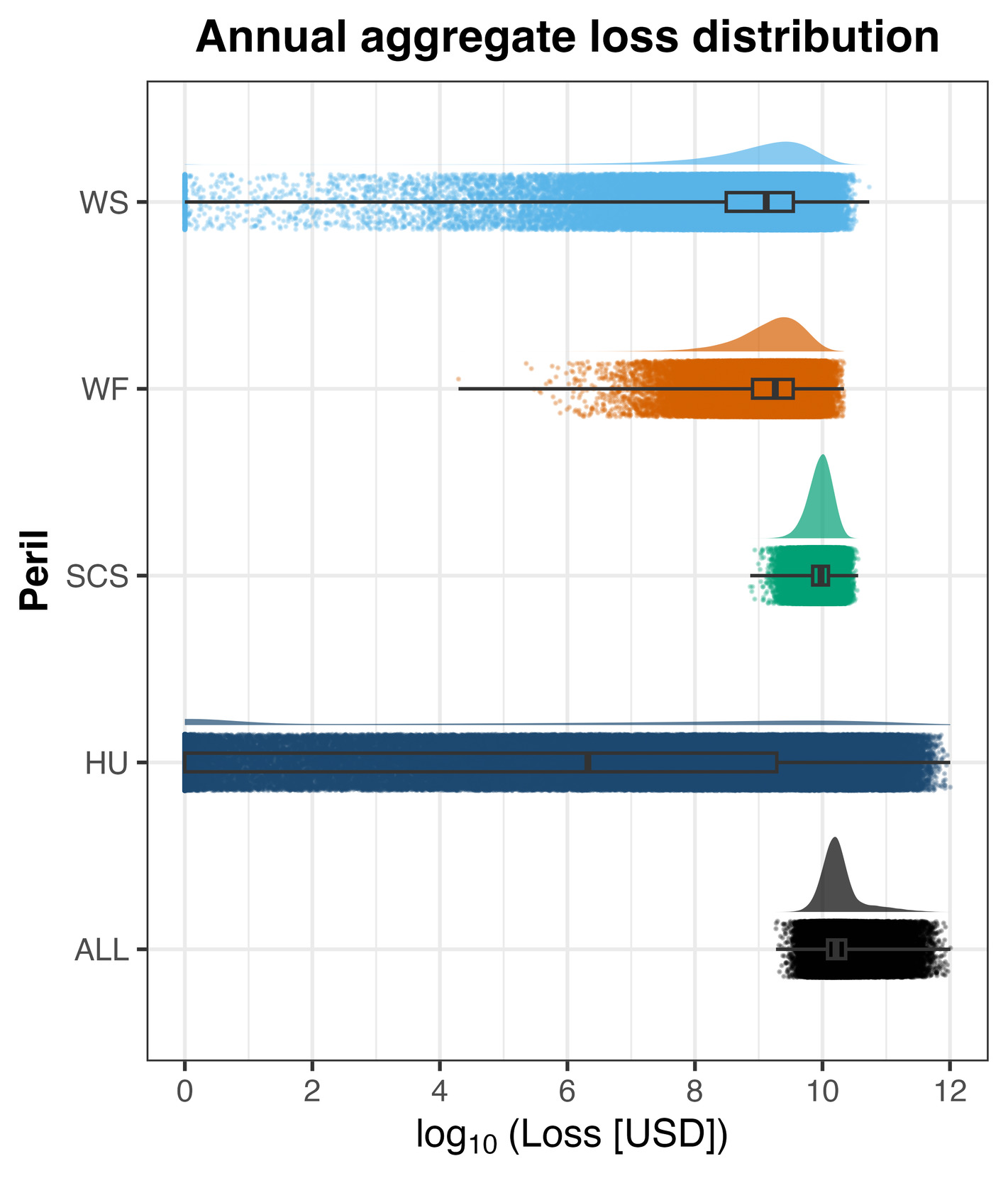
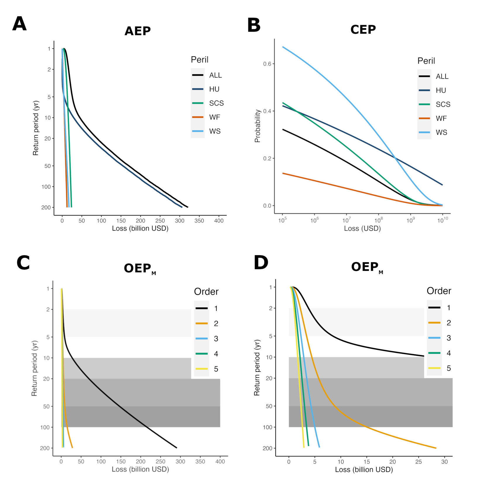
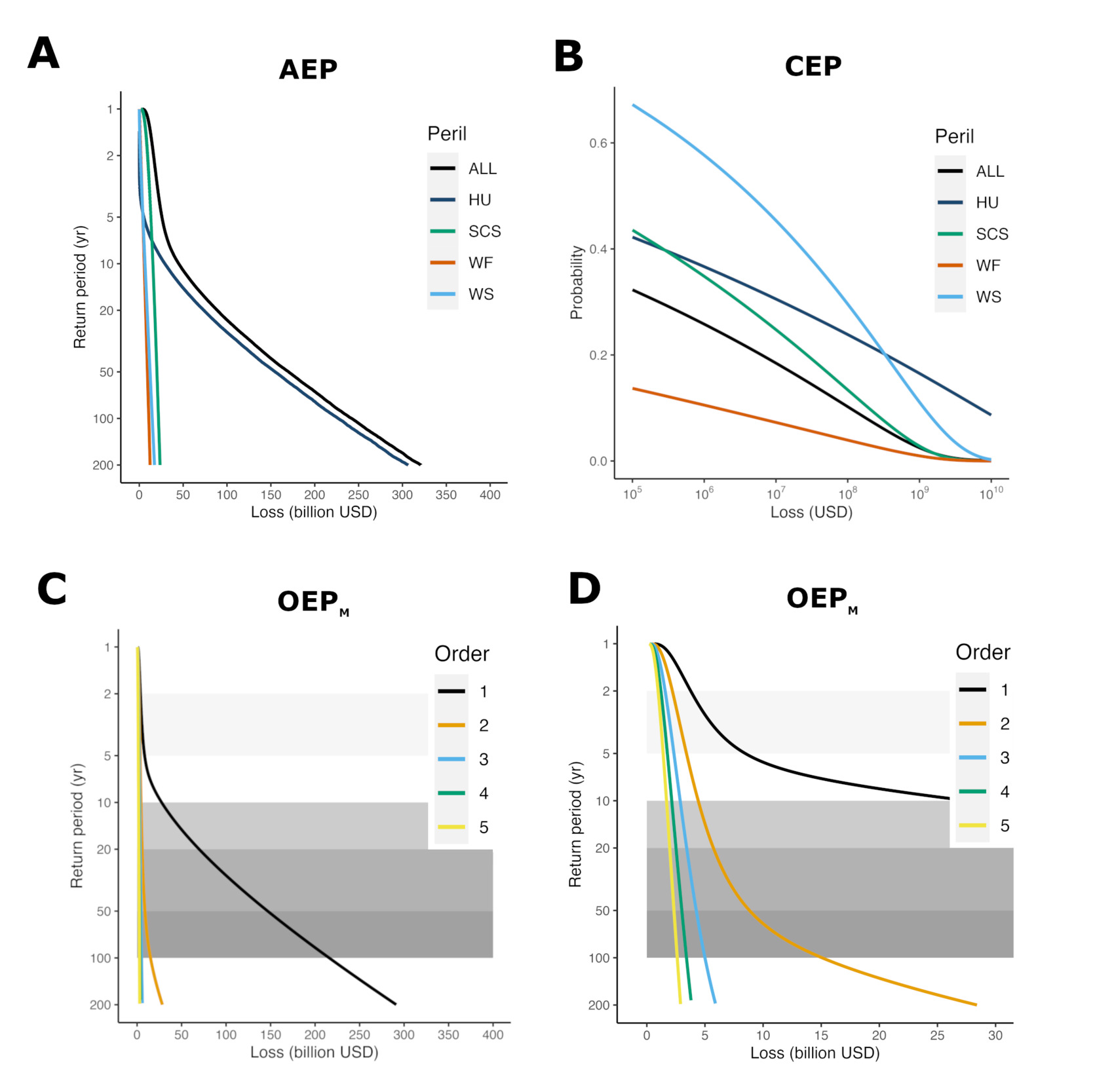
Figure 3 displays various exceedance probability (EP, defined as 1 minus the cumulative probability) curves obtained from our $S=500K$ year simulation (or by direct numerical integration in cases with analytical forms). Panels A, C, and D display return period on the vertical axis, which is the inverse of the EP. Panel A displays the annual aggregate EP for the multiperil model (ALL) and for each individual peril. Panel B displays the EPs of the multiperil severity, as well as the individual perils. Panel C displays the first five order statistic EPs for the multiperil model, as well as a blown up version in Panel D. Panel A makes clear the dominance of the HU peril to tail losses and suggests that contributions for layers with low attachments $$A$ should come from all perils. Panel B demonstrates the stark differences in the severities for each peril, showing that HU has high loss per event (high area under the curve, noting the log scale on the x-axis), and WF has high volatility (flat severity EP). Panel D shows that the annual maximum loss (Order 1) is expected to dominate higher layers (with high attachment $$A$), whereas the picture is more complex for lower layers (with low $$A$ and $$E$). In results to follow, we chose $$A$ and $$E$ by reading off loss thresholds consistent with particular return periods from the occurrence exceedance probability (OEP1), following what we believe to be common market practice.

Figure 3.Exceedance probabilities for various models. Panel A depicts the annual aggregate EP for the individual peril models, as well as the multiperil model denoted by ALL. Panel B depicts the EP of the individual severity distributions, as well as the multiperil model. Panels C and D depict the EP curves for order statistics up to $M=5$. Panel D is a zoomed in version of Panel C. This figure is identical to Figure 4 of Khare and Roy (2021) except for the earthquake peril, which is excluded.

3.2. Design of the numerical experiments and model perturbations

Broad scientific consensus is that anthropogenic climate change impacts both frequency and severity characteristics of natural catastrophe perils (Seneviratne et al. 2021; Calvin et al. 2023). Table 1 of Section 2.2 displays the various parameter choices associated with our base model. A natural question is how climate change will impact the parameterization in Table 1 and what effect this has on technical metrics. We do not tackle this question directly; rather, we choose to display results for reasonable ranges of model parameters, hoping to garner interesting insights about the impact climate change may have on various technical reinsurance perspectives.

Table 1 suggests an approach to generating perturbed model configurations by varying the AAL, the expected frequency for each peril $\mathbb{E}[N]$, and the peril severity mean and standard deviation (and hence CV). We chose to generate the perturbations by varying one peril at a time and quantifying the impact on catXL pricing metrics, keeping all other perils fixed to the base model configuration:

• Results are displayed across a range of perturbation factors $p_{1}\in[.5,1.5]$ and $p_{2}\in[.5,1.5]$

• Perturbation parameter $p_{1}$ simultaneously multiplies the AAL and $\mathbb{E}[N]$ with the same factor

• Perturbation parameter $p_{2}$ multiplies the standard deviation of the severity distribution

Our $p_{1}$ frequency parameter enables us to explore scenarios where the frequency and overall losses from AAL of a given peril changes in future states, exploring both $50\%$ decreases and increases. By choice, $p_{1}$ multiplies both AAL and $\mathbb{E}[N]$ simultaneously. This is motivated by the notion that future states with higher frequency are also likely to incur higher AALs due to economic exposure growth. Our $p_{2}$ perturbations reflect future states with $50\%$ increases or decreases in severity volatility (which are intended to capture a range of possible outcomes under climate change). By design, our model perturbations do not change the mean of the peril severities (or the combined model). We generated numerical results for a variety of low and high catXL layers where the attachment $$A$ and exhaustion $$E$ were chosen to be consistent with following return period thresholds (from the OEP1 of the multiperil base model): 0–2, 2–5, 5–10, 10–20, 20–50, and 50–100 years return period. Our layer definitions are designed to mimic typical industry practice as much as possible to make our results relevant for practitioners. To quantify the impact of reinstatements, we generated results for $n\in[0,1,2,4,8,16]$ and the unlimited case with $n\rightarrow\infty$. Results to follow are displayed in a space where the y-axis is proportional to $p_{2}$ and the x-axis is proportional to $p_{1}$ using contour plots of $\mathbb{E}\left[Y_{AE}\right]$, $\mathbb{S}\left[Y_{AE}\right]$ and their sum.

3.3. Numerical accuracy of discrete Fourier transform calculations of technical pricing metrics

The pricing metrics discussed in this work were computed using the FFT implementation outlined in Section 2.4.2 and detailed in Appendix C. For all results we set the maximum modeled loss to $L_{max}=\$10,000$ billion and used a uniformly spaced grid of dimension $M=2^{25}>33e6.$ This implies a grid spacing of approximately $0.000298$ billion dollars, orders of magnitude smaller than the mean losses per event for the high frequency, low severity perils WF ($\approx0.035$ billion dollars) and SCS ($0.1$ billion dollars) (base model configuration). To assess numerical accuracy we used benchmarks obtained using the integrals in Appendix A (pre-catXL) and Appendix B (post-catXL). Numerical integrals were computed using a standard python NumPy package. We deemed integration errors to be at most 1e-8. Independent code was developed in R achieving nearly identical results. The numerical integration results are therefore suitable benchmarks for the FFT results. We used the percentage error and “equivalent simulation years” method discussed in Section 2.4.3. Results are displayed in Table 2 (base model).

The results in Table 2 show that our FFT implementation is accurate. For example, in the pre-catXL case, the AAL and standard deviation have errors of less than $0.1\%$ and yield an equivalent number of years of simulation, roughly $20e6$ years, much larger than in most practical settings (typically up to $1e5$ years). Low (0–2 RP) layer and high (50–100) layer results are accurate enough for our purposes. The higher layer errors are larger, likely from the lower attachment probability (consistent with our intuition). Since the results in Table 2 are for the base model configuration, we also tested the accuracy using various combinations of perturbations to the model as outlined in Section 3.2, yielding qualitatively similar accuracy (omitted for brevity). With assurance that our numerical scheme is accurate, we set the stage to present the core results.

3.4. Numerical results

First we present the results for a low and high catXL layer in the case of unlimited reinstatements ($n\rightarrow\infty$).

3.4.1. Low and high catXL layers: Unlimited reinstatements

The low layer loss thresholds are defined by the base model multiperil OEP1 from 0 to 2 years return period, with $$A=0$ and $$E=3.79204$ (billion), and the high layer is for the 50 to 100 years layer with $$A=146.763$ billion and $$E=215.837$ billion.

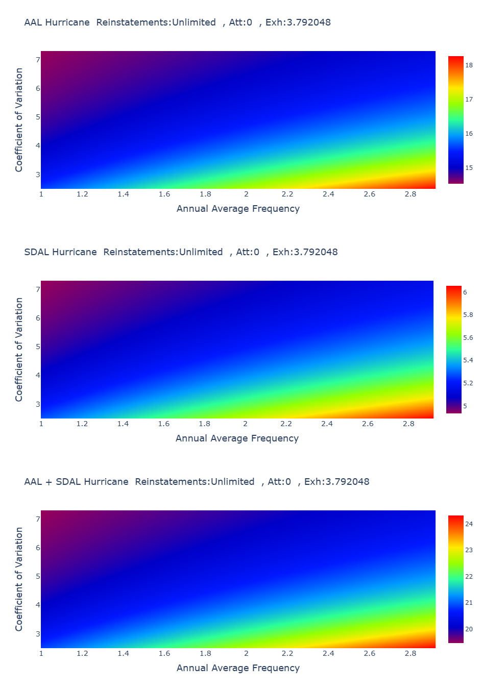
Figure 4 displays the low layer results for HU model perturbations ($n\rightarrow\infty$). The upper panel displays the $\mathbb{E}\left[Y_{AE}\right]$ (AAL) with $\mathbb{E}\left[N_{HU}\right]$ on the x-axis, and $CV$ for the HU severity on the y-axis (following our design in Section 3.2). The upper panel shows that increasing frequency drives up AAL (not surprisingly), but higher CV results in lower AAL. The middle panel displays results for the standard deviation $\mathbb{S}\left[Y_{AE}\right]$ in the same format, showing similar behavior to the AAL, and the lower panel displays the “risk metric” $\mathbb{E}\left[Y_{AE}\right]+\mathbb{S}\left[Y_{AE}\right]$, which amalgamates the upper and middle panel. Figure 4 demonstrates that the pricing metrics are indeed sensitive to HU model perturbations. The base model configuration is where $\mathbb{E}\left[N_{HU}\right]=2$ and $CV=5$, and we see that the risk metrics vary between (roughly) –5% and +20%.

Figure 4.Sensitivity results for the 0-2 RP low layer varying the HU model parameters only (all other parameters kept fixed). Results are for unlimited reinstatements $(n \rightarrow \infty)$. The upper panel displays the AAL with annual average frequency on the x-axis and CV of the severity on the y-axis. The size of the perturbations represent $50 \%$ upward and downward perturbations of the parameters in the base model configuration. The center panel displays results for the annual loss standard deviation, and the lower panel displays the risk metric (sum of AAL and standard deviation). The center of each panel represents results for the base model configuration.

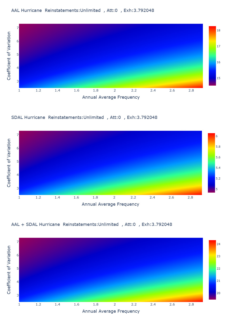
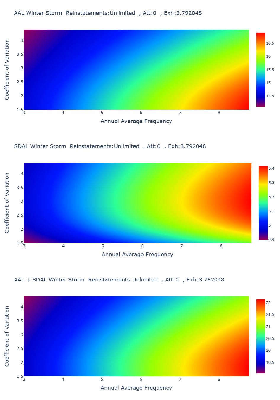
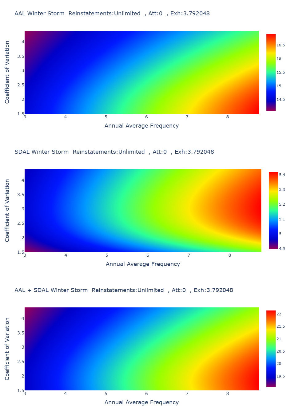
Figure 5 displays low layer results for WS perturbations. The results are similar to HU but the range of risk metrics is lower, and while increasing frequency always drives up $\mathbb{E}\left[Y_{AE}\right]$ and $\mathbb{S}\left[Y_{AE}\right]$, the effect of increasing CV for WS differs from that of the HU case. For example, the middle panel shows a convex relationship of $\mathbb{E}\left[Y_{AE}\right]$ with CV (opposite of Figure 4 for HU). Hence, no simple rule of thumb clarifies the effect of changing peril severity CV (for fixed frequency).

Figure 5.Low layer results for WS perturbations. This figure displays the analogous results to Figure 4, except the WS (rather than HU) parameters are varied. The size of the upward and downward perturbations relative to the base model configuration for WS are the same as in Figure 4 (50%). The center of each panel represents results for the base model configuration.

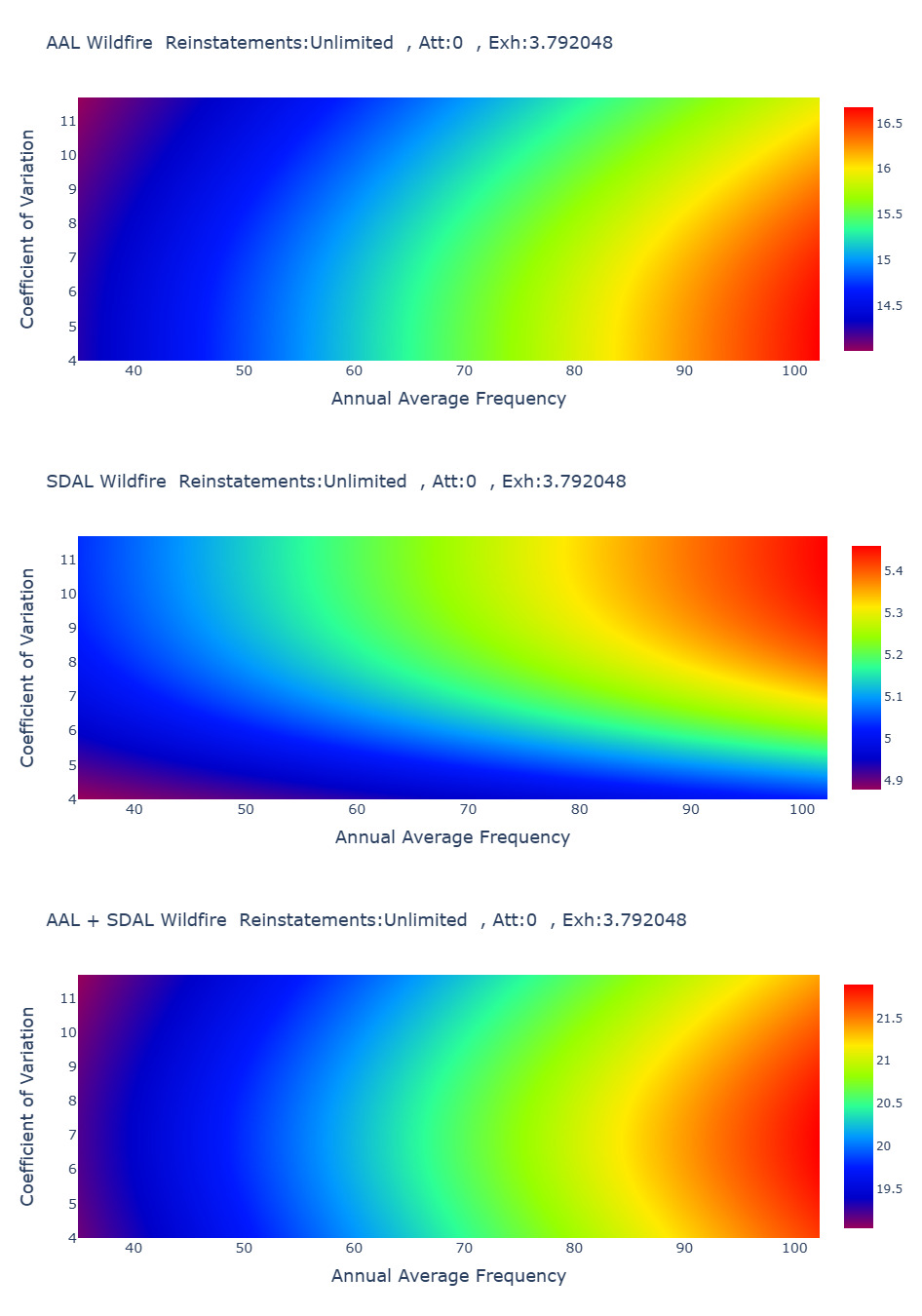
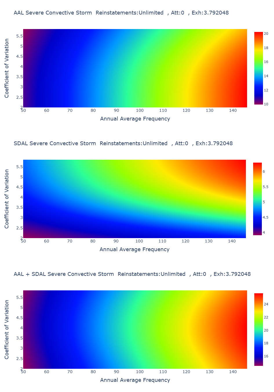
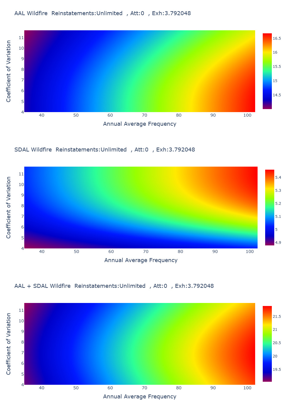
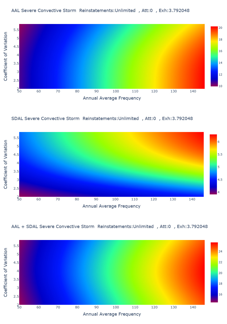
Figures 6 and 7 display analogous low layer results for WF and SCS perturbations, respectively. The results are qualitatively similar to those of the HU (Figure 4) and WS (Figure 5) cases but differ in the details. Figure 7 demonstrates that the results are most sensitive to changes in the specification of the SCS model parameters. The bottom panel shows an expanded range risk metric (–25% to +20%) compared with that of HU (–5% to +20%).

Figure 6.Analogous low layer results for WF perturbations. This figure also displays the analogous results to Figure 4, except the WF (rather than HU) parameters are varied. The size of the upward and downward perturbations relative to the base model configuration for WF are the same as those of the HU in Figure 4. The center of each panel represents results for the base model configuration.

Figure 7.Analogous low layer results for SCS perturbations. This figure displays the analogous results to Figure 4, except the SCS (rather than HU) parameters are varied. The size of the upward and downward perturbations relative to the base model configuration for SCS are the same as for those of HU in Figure 4. The center of each panel represents results for the base model configuration.

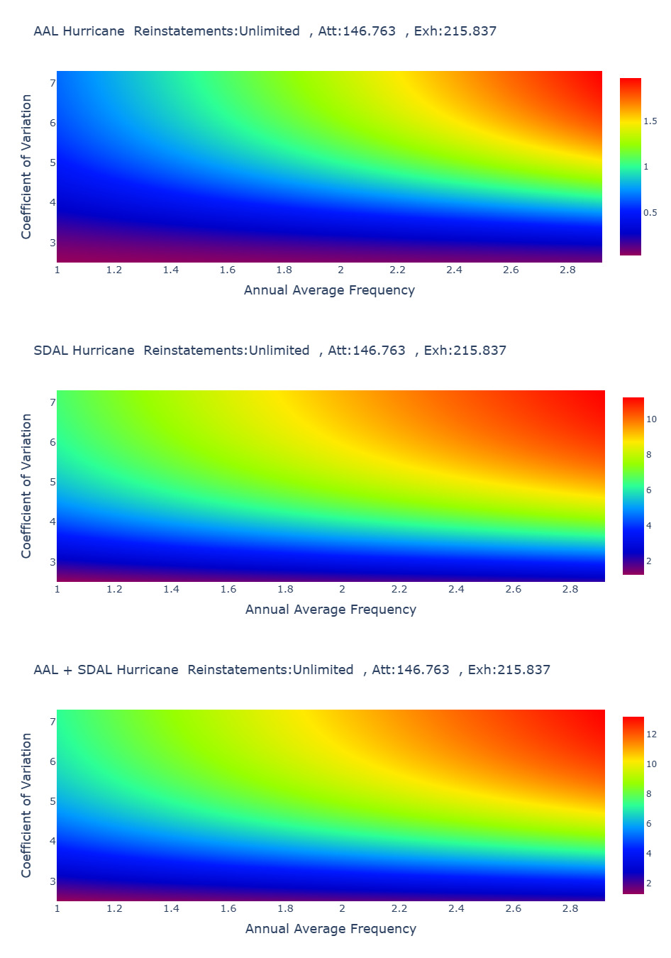
We now move to the high layer ($n\rightarrow\infty$). Figure 8 displays results for HU (analogous to Figure 4). The results are starkly different to the low layer. First, we see that increasing HU CV increases the AAL, $\mathbb{S}\left[Y_{AE}\right]$ and the risk metric (opposite to the effect seen in Figure 4). We also see that for the base model configuration, the ratio of $\frac{\mathbb{S}\left[Y_{AE}\right]}{\mathbb{E}\left[Y_{AE}\right]}$ in high layer case (7) is around 20 times the value for the low layer (1/3). The high layer losses are significantly more volatile (not surprisingly). The high layer also exhibits extreme sensitivity to the HU model perturbations, as revealed by the lower panel of Figure 8 (-85% to +70%). This range is much higher than our results for the low layer (-5% to +20%).

Figure 8.Sensitivity results for the 50 to 100 RP high layer varying the HU model parameters only (all other parameters kept fixed). Results are for unlimited reinstatements $(n \rightarrow \infty)$. The upper panel displays the AAL with annual average frequency on the x-axis and CV of the severity on the y-axis. The size of the perturbations represent $50 \%$ upward and downward perturbations of the parameters in the base model configuration. The center panel displays results for the annual loss standard deviation, and the lower panel displays the risk metric (sum of AAL and standard deviation). The center of each panel represents results for the base model configuration.

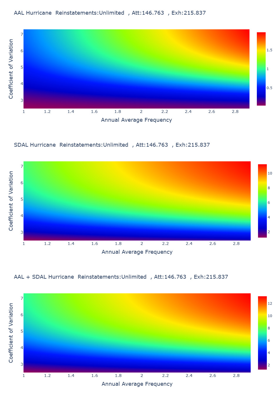
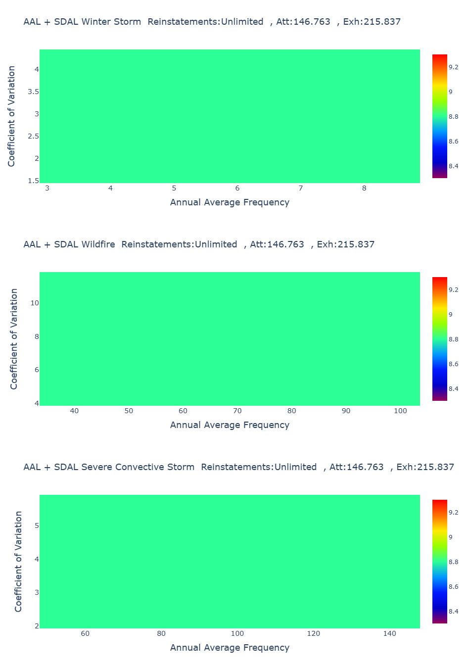
Figure 9 displays the risk metrics for the high layer experiments, with WS in the upper panel, WF in the middle panel, and SCS in the lower panel. Figure 9 implies nearly zero sensitivity to model perturbations for WS, WF, and SCS. This starkly contrasts the low layer results with nontrivial sensitivity to all peril perturbations. Apparently the losses from WS, WF, and SCS are simply not material enough to influence the losses to the high layer.

Figure 9.Sensitivity results for the 50 to 100 RP high layer varying the WS (upper panel), WF (middle panel), and SCS (lower panel). Each panel displays the risk metric (sum of AAL and standard deviation). The sensitivities are flat, showing nearly zero sensitivity to model assumptions for lower severity perils.

The unlimited reinstatement cases in Figures 4, 5, 6, and 7 (low layers) and Figures 8 and 9 (high layers) lead to the following summary:

• Low layers have the following properties: (1) Low volatility for annual losses (standard deviation per unit AAL); (2) Sensitivity to all four perils—with highest sensitivity from HU and SCS; (3) Increased risk metric (for fixed CV) at higher frequency, while the relationship with CV is peril dependent; and (4) A range of –25% to 20% in the risk metric.

• High layers have the following properties: (1) Annual losses are highly volatile; (2) Results are highly sensitive to HU model perturbations with (nearly) zero sensitivity to WS, WF, and SCS; (3) Risk metric is increased with frequency and CV (for HU); and (4) Sensitivity to HU model perturbations is high, with a range of –85% to 70% in risk metric.

The above results represent two extremes on a spectrum. There are clear trade-offs. We now explore the effects of adding finite reinstatements.

3.4.2. Low and high catXL layers: Finite reinstatements

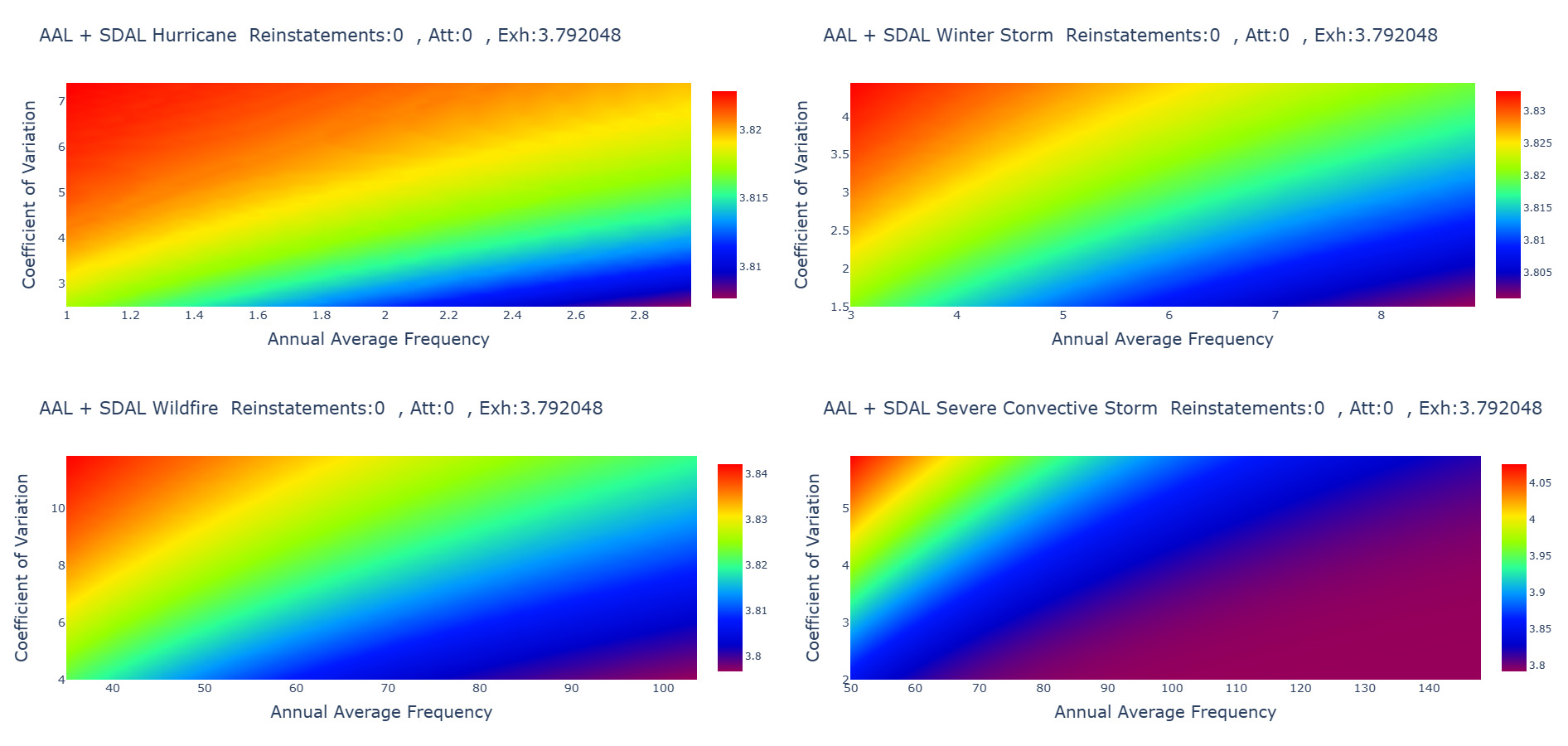
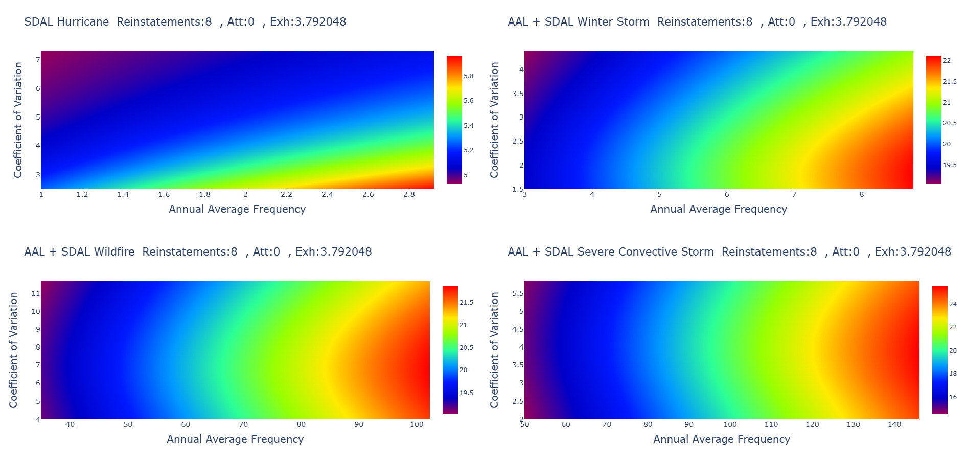
Figure 10 displays low layer results with $n=0$. The upper left panel displays HU, the upper right shows WS, the lower left shows WF, and the lower right show SCS. With $n=0$, the aggregate limit is $A_{lim}=(E-A)$. This annual loss cutoff has a dramatic effect on the range of risk metric sensitivity. For example, the range of risk metrics for HU in the upper left is very close to the base model configuration with $\lambda_{HU}=2$ and $CV=5$. Qualitatively, the results for WS, WF, and SCS are similar. We also note that the risk metric itself is a factor of 6 lower than the case with $n\rightarrow\infty$ (Figure 4), and the risk metric is only slightly larger than $(E-A)$. In fact, for the upper left panel HU results, $\frac{\mathbb{S}\left[Y_{AE}\right]}{\mathbb{E}\left[Y_{AE}\right]}\approx0.005$, compared with $1/3$ in the $n\rightarrow\infty$ limit (similar results for WS, WF, and SCS). For the low layer, including the reinstatement, ($n=0$) nearly eliminates model sensitivity and annual loss volatility.

Figure 10.Sensitivity results (for the risk metric) for the low layer (0–2 RP) case where the catXL contract has $n = 0$ reinstatements. In stark contrast to Figures 4, 5, 6, and 7 for unlimited reinstatements, the above results show very low sensitivity to model assumptions.

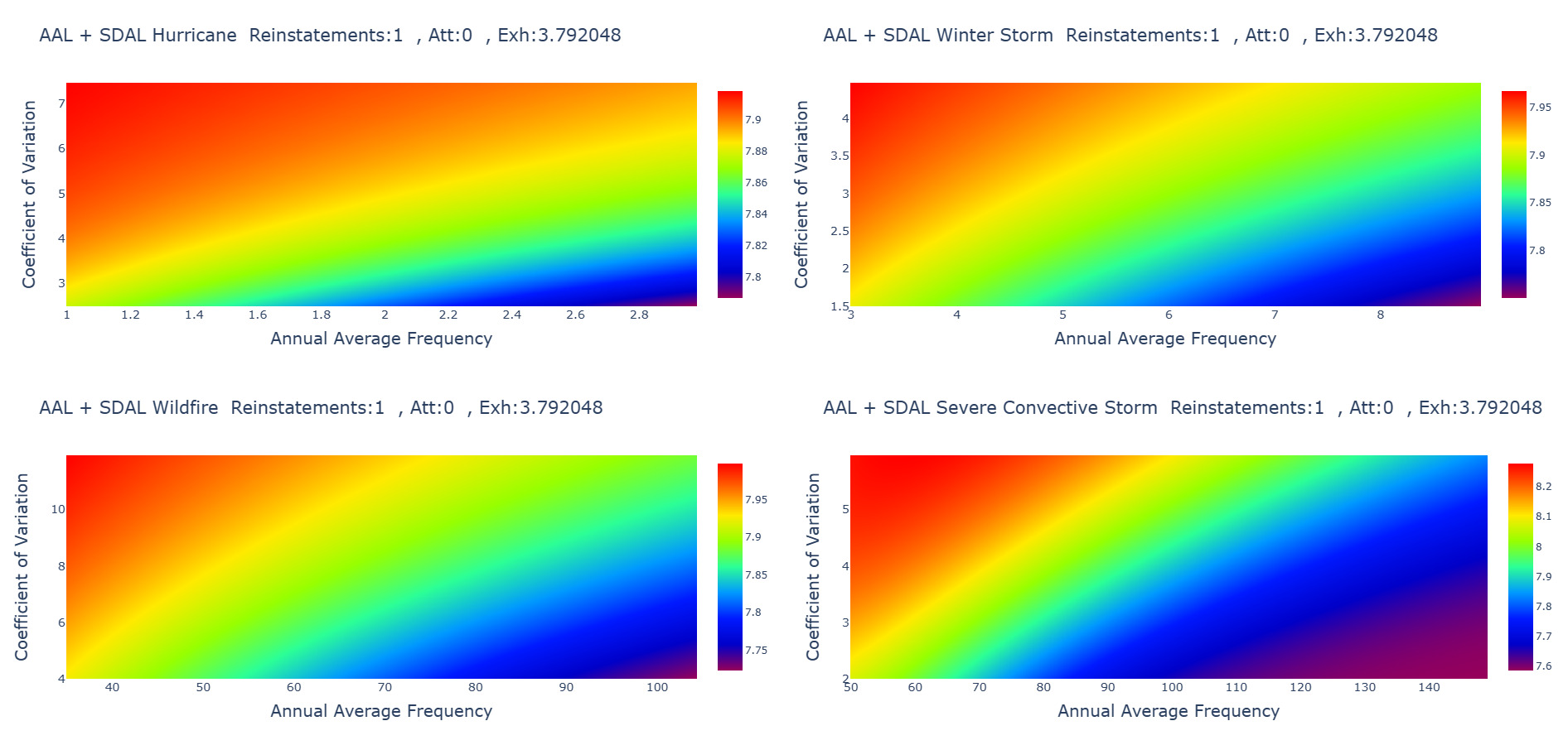
Figure 11 displays the analogous results to Figure 10, but for the case where $n=1$ and the aggregate limit $A_{lim}=2(E-A)$. Comparing Figure 11 with Figure 10, we see a larger range of risk metrics and more annual loss volatility for which $\frac{\mathbb{S}\left[Y_{AE}\right]}{\mathbb{E}\left[Y_{AE}\right]}\approx0.05$ (10 times the $n=0$ case, and similar for other perils). Adding reinstatements drives up model sensitivity and annual loss sensitivity. We expect this trend to continue as we add reinstatements.

Figure 11.Analogous to Figure 10 but for the case where the number of reinstatements $n=1$. Compared with the $n=0$ case in Figure 10, the results demonstrate a higher range of risk metrics and therefore higher sensitivity.

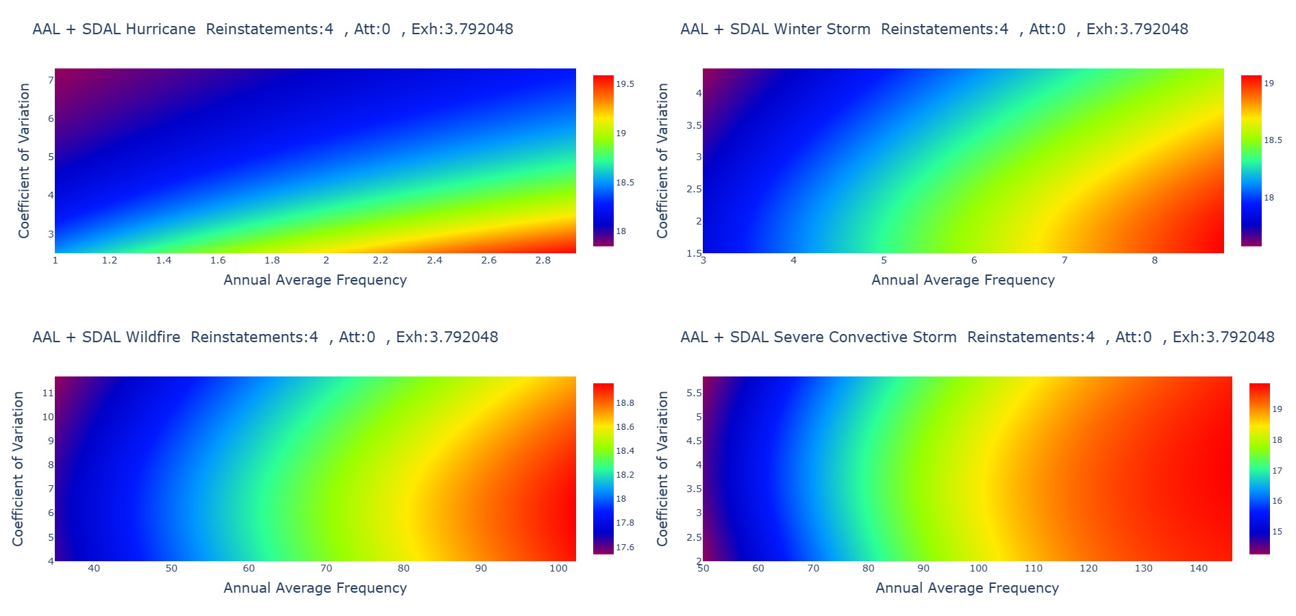
Figures 12 and 13 display low layer results for $n=4$ and $n=8$, respectively, and demonstrates the trend discussed above that increasing the number of reinstatements enables higher model sensitivity and volatility ($\frac{\mathbb{S}\left[Y_{AE}\right]}{\mathbb{E}\left[Y_{AE}\right]}$ for $n=4$ is slightly less $n=8$, which is very close to the $n\rightarrow\infty$ case). The annual loss volatility appears to “saturate” once we reach $n=8$.

Figure 12.Analogous to Figures 10 and 11 but with the number of reinstatements $n=4$. These results demonstrate that as the aggregate limit is increased we enable a higher sensitivity to model assumptions.

Figure 13.Analogous to Figures 10, 11, and 12 with the number of reinstatements set to $n=8$. These results demonstrate that increasing numbers of reinstatements lead to higher sensitivity of the risk metric to model assumptions and yield similar sensitivity as that exhibited in the unlimited reinstatements case in Figures 4, 5, 6, and 7.

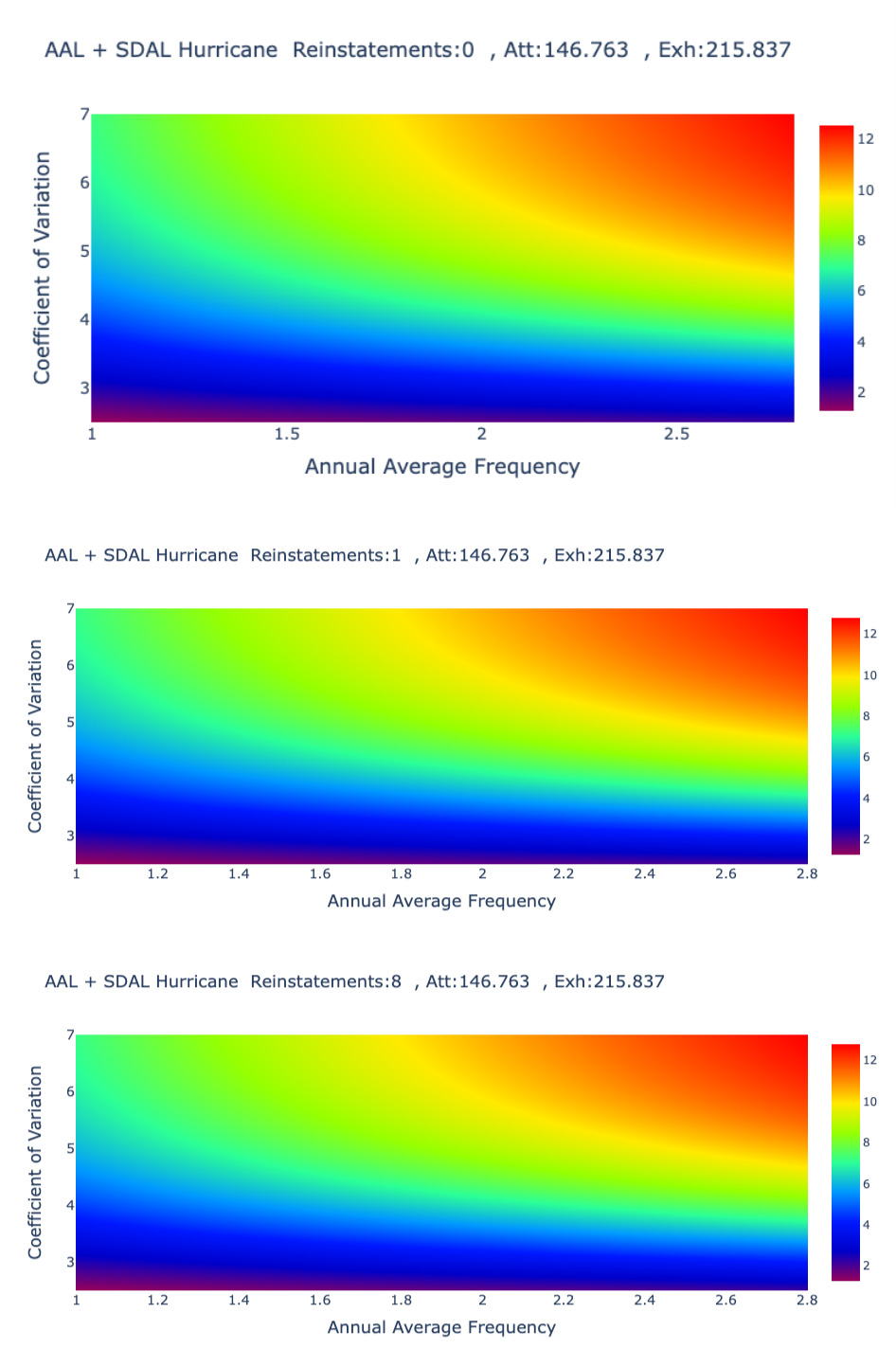
Results for the high layer are depicted in Figure 14, which shows HU with $n=0$ reinstatements in the upper panel, $n=1$ in middle panel, $n=8$ in the bottom panel. In stark contrast to the low layer, reinstatements have little to no effect on the volatility and/or model sensitivity of the high layer (we omitted results for other perils as there is no sensitivity even in the case for $n\rightarrow\infty$ as shown in Figure 9). For the high layer, reinstatements are not an effective “control” mechanism.

Figure 14.Results for the high layer ( $50-100 \ \mathrm{RP}$ ) varying HU model parameters for varying numbers of reinstatements ranging from $n=1$ in the upper left panel to $n=8$ in the lower right panel. The range of risk metrics in the above four panels is similar to the range seen in Figure 8 for the unlimited reinstatements case. The inclusion of reinstatements has little effect on the range of risk metrics obtained by varying model parameters.

3.4.3. Intermediate layers

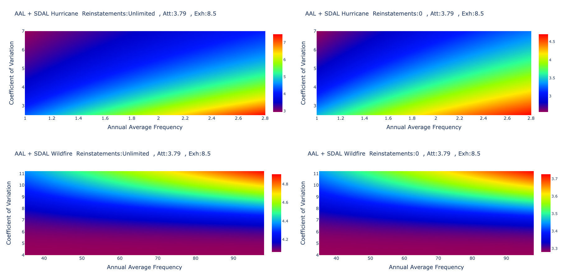
To this point, we have presented results for (extreme) low and high layers under varying numbers of reinstatements. Our results suggest a progression from low to high layers when we consider model sensitivity, annual loss volatility, which perils are important (peril uncertainty), and the effect of varying the reinstatements $n$. We therefore expect the progression to evidence itself when we look at “intermediate layers” lying between the low and high layers. Figure 15 displays risk metric sensitivity for the 2 to 5 year layer where $$A=3.79204$ and $$E=8.5$ (billion). The upper left displays results for HU where $n\rightarrow\infty$ and the upper right for $n=0$. The lower left displays results for WF with $n\rightarrow\infty$ and lower right with $n=0$. Our results show the progression discussed above. As for the $n=0$ case, the risk metric is more sensitive to HU than for WF, and the effect of including a reinstatement is slightly damped. Qualitatively similar results to those of WF are achieved for WS and SCS (omitted for brevity).

Figure 15.Risk metrics for the 2 to 5 year intermediate layer. The upper left panel has HU in the $n \rightarrow \infty$ case. The upper right displays the $n=0$ case, showing a notable impact on the risk metric but not as extreme as with the low layer. The bottom two panels show the analogous results for WF.

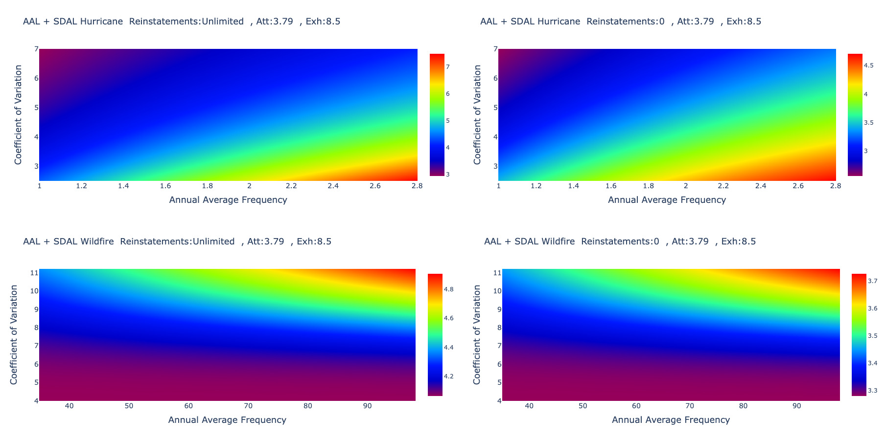
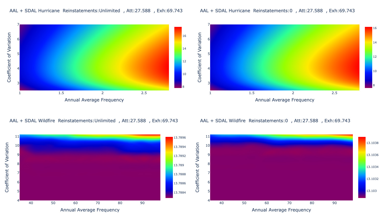
Figure 16 displays results analogous to Figure 15, except for the 10–20 year layer from $$A=27.588$ to $$E=68.743$ (billion). Figure 16 gives more evidence for the progression in that we see high sensitivity to HU, little to no sensitivity for WF, and very minimal impact from finite reinstatements.

Figure 16.The 10–20 year intermediate layer in the same format as Figure 15. The figure shows increased sensitivity to HU and diminished sensitivity to WF perturbations. In comparison with Figure 15, Figure 16 shows diminishing impact from the inclusion of finite reinstatements.

3.4.4. Key findings from the numerical experiments

Sections 3.4.1, 3.4.2, and 3.4.3 explored various dimensions important to formulating technical pricing metrics of catXL layers: peril model parameter uncertainty, the return periods associated with a given catXL layer, and the number of reinstatements constraining the annual aggregate loss. Our results suggest some general principles useful for reinsurers dealing with model perturbations.

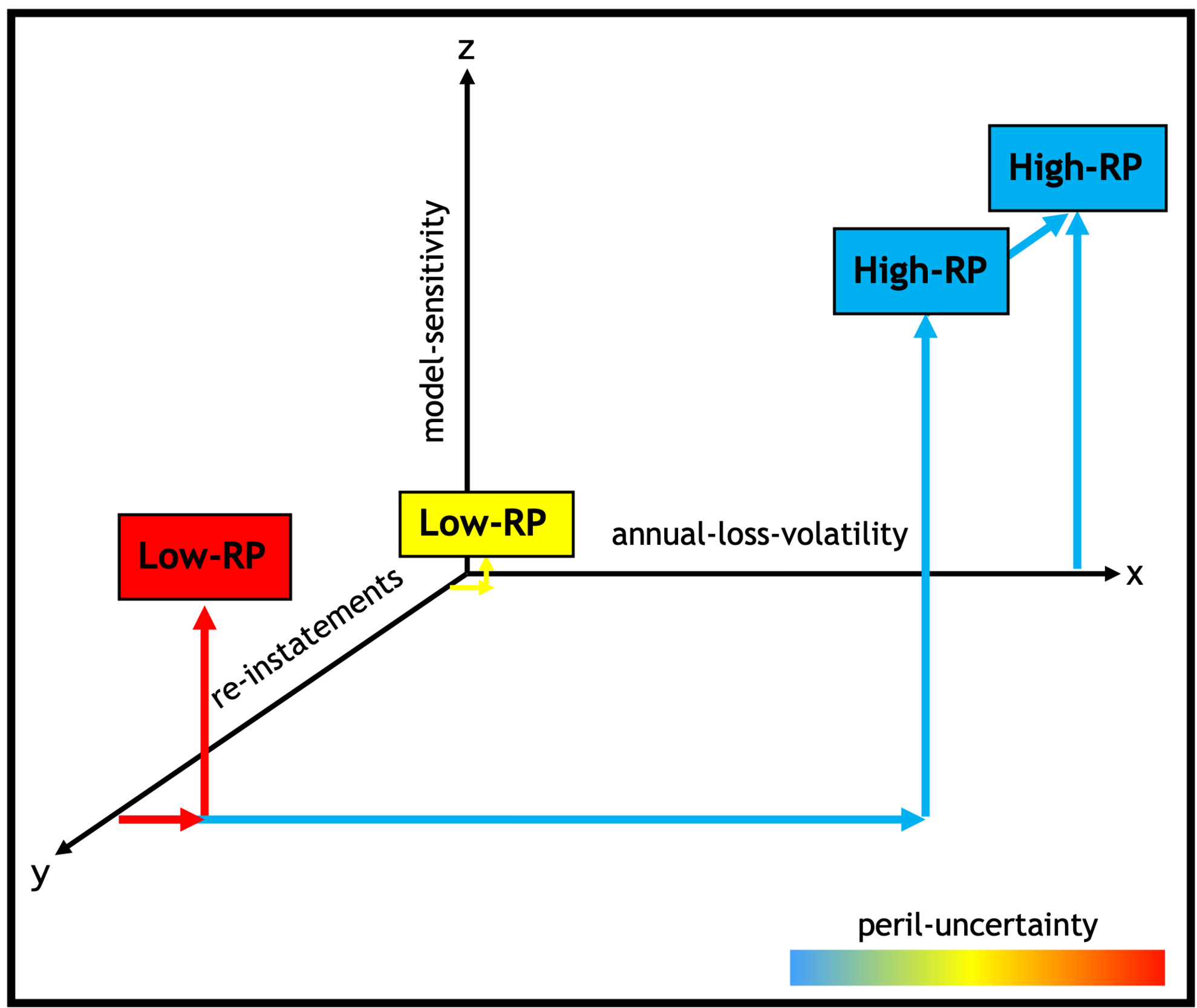
Figure 17 provides a visual aid to clarify our results. The x-axis depicts the annual loss volatility $\frac{\mathbb{S}\left[Y_{AE}\right]}{\mathbb{E}\left[Y_{AE}\right]},$ the y-axis shows the number of reinstatements for a given catXL layer, and the z-axis shows model sensitivity (the change in risk metric under model perturbations). Our result for the low layer with large ($n\rightarrow\infty$) number of reinstatements is represented by the red “low-RP” box. This result is characterized by low annual loss volatility, moderate model sensitivity, and high peril uncertainty (the risk metric is sensitive to all four perils). The yellow “low-RP” for small $n$ is characterized by (near zero) low volatility and model sensitivity and moderate peril uncertainty. Higher frequency drives up the risk metric, but the effect of increasing severity CV is peril dependent. The other end of this spectrum shows the high layer results indicated by the two blue “high-RP” boxes, which are characterized by high model sensitivity, high annual loss volatility, but low peril uncertainty (only sensitive to HU changes). The high layer results are not sensitive to the inclusion of finite reinstatements. For high layers, higher HU frequency and CV drive up the risk metric. The intermediate layer results in Section 3.4.3 fit nicely between the two extreme cases, as we would expect.

Figure 17.A qualitative depiction of the numerical results. The x -axis depicts the annual loss volatility $\frac{\mathbb{S}\left[Y_{A E}\right]}{\mathbb{E}\left[Y_{A E}\right]}$, the y-axis shows the number of reinstatements $n$, and the z-axis shows the model uncertainty reflecting the range of risk metrics for a given catXL contract layer. The red “Low-RP” box depicts the case with large $(n \rightarrow \infty)$ reinstatements for the low layer with $$A=0$ and $$E=3.79204$ (billion). The yellow “Low-RP” box depicts low layer results with $n=0$ reinstatements. Two high layer cases are depicted in the blue “High-RP” boxes. Both model uncertainty and annual loss volatility are (nearly) the same for the two “High-RP” cases, as variation in the number of reinstatements has little quantifiable impact. Peril uncertainty is indicated by the color spectrum in the lower right and quantifies the number of perils of the four perils (HU, WS, WF, and SCS) that influence model uncertainty for a given case (blue indicates low peril uncertainty).

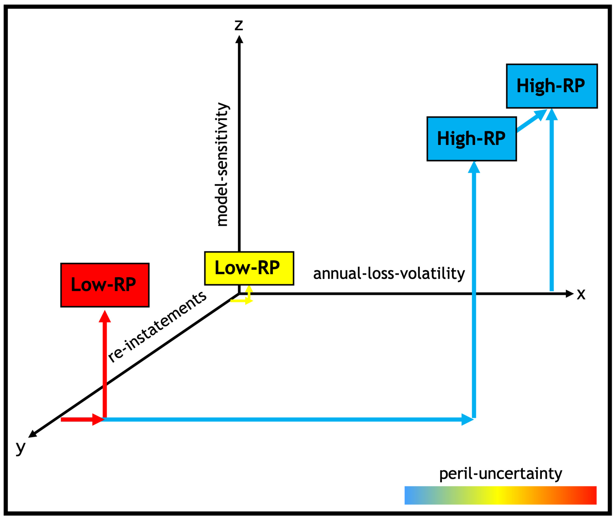
Our results demonstrate clear trade-offs if reinsurers shift from low to high layers (or vice versa). With large numbers of reinstatements, the transition from low to high layers drives up model sensitivity and annual loss volatility. This increase in model sensitivity and annual loss volatility is “traded” for lower peril uncertainty. Including reinstatements can control model sensitivity and annual loss volatility, but only for low layers. We note that the risk metric relationship to changes in severity CV also changes as we move from low to high layers (from peril dependent to positive dependence on only HU CV for the high layer). Section 4 discusses the implications of our technical results for reinsurance strategies under climate change and provides context for recent market dynamics (as of 2024).

4. Summary and Conclusions

This paper presents a set of numerical experiments using a representative natural catastrophe risk model consisting of four climate perils (HU, WS, WF, and SCS). The base model (Section 2.2) is designed to mimic a US-wide insurance portfolio with realistic relativities across perils. Section 3.4 presents a set of sensitivity analyses where we vary model parameters (related to frequency and severity) for each peril independently. These sensitivity results are motivated by the notion that climate change represents perturbations to the natural catastrophe models used by reinsurers to formulate technical metrics that inform catXL pricing. We have systematically varied catXL contract parameters: (1) Attachment $$A$ and exhaustion $$E$ representing typical low, intermediate, and high layers in the market; and (2) number of reinstatements $n$. Our chosen technical metrics are the layer AAL and standard deviation (and their sum) motivated by market practice. Insofar as our top-down catastrophe model is relevant to the market, our results yield a number of new and fundamental insights. We find a stark contrast between reinsurance metrics for low (where $$A$ and $$E$ represent low return periods) and high (vice versa) catXL layers. For the specific US nationwide portfolio and four-peril representative model studied in this work, the main technical conclusions are stated below.

Low layer results are characterized as follows:

• Technical metrics exhibit low annual loss volatility (per unit AAL), moderate sensitivity to model parameter perturbations, and high sensitivity to all perils (high peril uncertainty) for unlimited reinstatements $(n \rightarrow \infty)$
• Finite reinstatements drastically reduce annual loss volatility and model sensitivity, and moderate peril uncertainty
• Higher frequency drives up the risk metric (as expected), but the relationship with severity CV is peril dependent

High layer results are characterized as follows:

• For unlimited reinstatements, technical metrics exhibit high (20x low layers) annual loss volatility, high sensitivity to model perturbations, and low peril uncertainty (since only HU model perturbations are meaningful)
• Finite reinstatements have no measurable impact on annual loss volatility and model sensitivity
• Higher HU frequency and CV drive up the risk metric

Our results for the low and high layers represent two ends of a spectrum. We have demonstrated that “intermediate layers” (with attachment $$A$ and exhaustion $$E$ lying between our chosen low and high layers) fit logically within this spectrum. Therefore, as we progress from low to high layers we see higher annual loss volatility, higher sensitivity to model parameter perturbations and less peril uncertainty.

The above conclusions yield practical insights for reinsurers whose portfolios are well approximated by a proportional slice of the US nationwide industry portfolio for the specific perils studied here. Logically, our results are most relevant for large reinsurers with significant market share in the US. While our study covers a use case of broad interest, the computational framework we have developed in this paper is of value to a broader set of portfolios and combinations of perils. The sensitivity analysis we used is conceptually simple and could be carried out by skilled actuaries and/or catastrophe risk analysts. Ideally, commercial and/or open source software would be available to perform the type of analysis presented in this paper. We also emphasize that our results are specific to the case where there are four covered perils (hurricane, winter storm, wildfire, and severe convective storm). In this work the peril uncertainty is negligible as we shift to higher layers. This is dependent on our specific modeling setup. For example, if we had included earthquake (although not strongly influenced by climate change) we would expect higher layers to be affected by both hurricane and earthquake. Also, under climate change, the relative importance of different perils may change, and could increase/decrease peril sensitivity in higher layers.

Despite the specificity of our results to a US nationwide portfolio subject to HU, WS, WF, and SCS, it is useful to ask how our results influence how we think about reinsurance strategies under climate change. Clearly, formulating an optimal reinsurance strategy under climate change is a profound and multifactorial problem. Our reductionist approach, which focused on technical metrics and a specific case, is one useful step forward. For example, suppose as a reaction to climate change, a reinsurer decides to tilt their portfolio to lower layers, believing that tail risk is too uncertain under climate change. Our results imply lower annual loss volatility and model sensitivity. We also gain a degree of “control” if we limit the number of reinstatements (lowering both volatility and model sensitivity). However, a clear trade-off is made for higher peril uncertainty. In this scenario, the reinsurer must model all four perils accurately, and this complexity is amplified by uncertainties from climate change. This is a nontrivial consideration, given the nature of perils such as SCS, with small scale features. On the flip side, if the reinsurer decides to underwrite higher layers in reaction to climate change, the result is higher volatility and model uncertainty but minimal peril uncertainty (since only HU is important). The high model uncertainty could be problematic if the reinsurer does not have a good grasp of climate change effects on HU. Steering the portfolio in one direction or the other as strategy therefore comes with trade-offs. Our results make these trade-offs clear.

Our work also provides insight on recent property catastrophe market dynamics (2024). Rate on line for global property catastrophe is near all-time highs, with considerable increases from 5 to 6 years ago (Guy Carpenter 2024). In this environment, reinsurers have tightened their terms and conditions and shifted their portfolios to higher layers (broadly speaking). This has implications for both insurers (cedants) and reinsurers. Insurers are left with more retained risk in the lower layers; hence, increasing peril uncertainty (and lower volatility and model uncertainty). This raises the importance of complex perils such as WF, WS, and SCS for insurers. Market factors—such as pressure on ability to flex insurance rates due to regulation—exacerbate the complexity. For reinsurers, the move to higher layers introduces more volatility and model uncertainty (driven by HU). Reinsurers must ensure they are adequately compensated for this additional volatility, which may be amplified if the effects of near term climate change on HU are poorly quantified. Any near term market shock that puts downward pressure on reinsurance rate on line would be consequential for reinsurers.

Our work sets the stage for additional studies. To further address climate change, it would be useful to extend our study to the case where we specify a multivariate distribution for all the peril parameters. This requires scientific insight beyond the scope of this paper but would enable a probabilistic interpretation of our results. The present work could be generalized by varying several perils simultaneously (instead of one peril at a time as done here for simplicity). Our analysis can be made more complete and richer by including market factors such as how well reinsurers are compensated in premiums for the various catXL contracts studied in this work. To aid in such analyses, we note that commercially available climate change conditioned catastrophe risk models are available to allow reinsurers forward looking views of risk. Although we focused on the reinsurer point of view, it would be useful to extend our analysis to consider insurer retained risk. Finally, the framework presented in this work can be applied to a wide range of specific reinsurer portfolios, for different peril combinations, for exposures in the US and around the globe. The insurance industry plays a critical role in mitigating the worst economic effects of climate change, and the authors encourage further work. The relatively recent adoption of natural catastrophe modeling by the banking and investment sectors raises the stakes even further.