Quantile and Log-Quantile Least Squares for Robust-Efficient Fitting and Validation of Log-Location-Scale Loss Models

Dedication. This paper is dedicated to the memory of Professor Ričardas Zitikis—a dear friend, an inspiring mentor, and a brilliant researcher—who over the years has shared many insights about the effectiveness of quantiles in economics, finance, quantitative risk management, and other fields.

1. Introduction

Claim severity models help insurance companies assess risk, set appropriate premiums, and ensure they have enough reserves to cover potential claims. Given that such models cannot be constructed without making assumptions, which may be reasonable but not perfectly correct, their estimation must be resistant to various potential violations of such assumptions. In other words, the model fitting techniques and validation tools must help actuaries to manage “model risk.” Among many manifestations of model risk, outliers are the most influential, evasive, and potentially harmful for ensuing applications. Therefore, robust-efficient fitting of these models is crucial because it yields accurate estimates of risk, even in the presence of outliers or imperfect data.

The literature on robust statistics is well established and offers a rich variety of techniques for robust-efficient fitting of parametric models. These are summarized in books by Hampel et al. (1986), Maronna et al. (2006), and Huber and Ronchetti (2009). In actuarial science, robustness studies have been conducted by many researchers who rely upon varying interpretations of robust models. For example, using the traditional interpretation (as defined in the aforementioned books), several authors worked to develop more robust credibility models, including Künsch (1992), Gisler and Reinhard (1993), Dornheim and Brazauskas (2007, 2011, 2013), Kim and Jeon (2013), and Zhao and Poudyal (2024). Robust-efficient estimation of heavy-tailed models was explored by Brazauskas and Serfling (2000), Serfling (2002b), Brazauskas et al. (2009), Zhao et al. (2018), and Fung (2022, 2025). And Poudyal (2021a, 2021b) extended robust methods to insurance payment data (e.g., left-truncated and right-censored data). Other interpretations of robustness have also been used in actuarial research. For example, adopting the minimum distance approach (i.e., the distance between probability distributions as presented by Basu et al. (2011)), robust risk analysis of several actuarial problems was conducted by Blanchet et al. (2019). Yet another approach is to incorporate distributional robustness by investigating the worst- and best-case scenarios for risk measures. Recent examples of this include Liu and Mao (2022) and Bernard et al. (2024), among many others. The methodology proposed in this paper relies upon the traditional interpretation of robustness.

Many loss severity distributions are special cases of the log-location-scale family, with the lognormal and Pareto-\(I\) distributions being the most prominent examples. The latter distribution also serves as a primary example of infinite-mean models that often present challenges in risk management (see Chen and Wang (2025) for an extensive review). This paper builds upon the work of Adjieteh and Brazauskas (2025) for location-scale families and constructs nonlinear and linear regression frameworks to estimate and validate log-location-scale distributions, which we accomplished by using two asymptotic results—the joint normality of sample quantiles of independent and identically distributed (i.i.d.) random variables and the delta method. Within these frameworks, we introduce four equally robust estimators—ordinary and generalized quantile (oQLS and gQLS) and log-quantile (log-oQLS and log-gQLS) least squares. The novelty of the proposed methodology lies in exploiting the asymptotic structure of the covariance matrix of sample quantiles, which is used to construct more accurate estimators. The new estimators offer attractive robustness-efficiency trade-offs and exhibit other appealing properties, such as their direct applicability to any log-location-scale distribution and their low computational costs. Specific contributions of this paper to advancing quantile least squares (QLS) methodology include the following:

• It introduces a nonlinear quantiles-based regression framework, which is valid for general loss models, and develops a log-linear approximation of its solution for the parameters of log-location-scale distributions.

• It extends the aforementioned approximation for Weibull and Pareto \(I\) models, for which the logarithmic transformation of quantiles does not isolate the parameters of interest. Thus, deriving log-oQLS/log-gQLS and their properties requires further work (see Section 2.4).

• It explores quantile-selection strategies and their effect on the estimators’ accuracy.

• It proposes a new model-based outlier-screening rule, tests its effectiveness using simulated and real data examples, and compares it with the effectiveness of some existing rules.

The rest of the paper is organized as follows. Section 2 introduces nonlinear and linear regression models based on sample and theoretical quantiles and log-quantiles. Then we define the oQLS/gQLS and log-oQLS/log-gQLS estimators for log-location-scale distributions and compare them using simulations. Further, we investigate robustness and efficiency properties of the log-QLS estimators and search for optimal quantile-selection designs. We complete the section by constructing a goodness-of-fit test for model validation. Section 3 describes simulation studies we conducted to verify the log-oQLS and log-gQLS estimators’ performance under data contamination and their effectiveness when applied to several outlier-screening rules. This section also investigates the power properties of the goodness-of-fit test. Section 4 examines the practical performance of the new estimators and the goodness-of-fit test using real data. Section 5 provides a summary and concluding remarks.

2. Quantile least squares

This section presents a general formulation of the QLS estimators for parametric distributions with the support on \((0, \infty)\). Two approaches are considered: the QLS based on raw quantiles, which results in nonlinear regression, and the log-QLS based on logarithmically transformed quantiles, which results in linear regression. Under both regression frameworks, two types of estimators—ordinary and generalized least squares—are studied for the class of log-location-scale families. Then we compare the QLS and log-QLS using several statistical and computational metrics. Further, we establish and illustrate asymptotic robustness and efficiency properties of the log-QLS estimators. Finally, we construct a goodness-of-fit test to validate the models fitted by log-gQLS.

Suppose a sample of i.i.d. positive continuous random variables, \(X_1, \ldots, X_n\), is observed. Let the cumulative distribution function (cdf) \(F_{\pmb{\theta}}\), probability density function (pdf) \(f_{\pmb{\theta}}\), and the quantile function (qf) \(F^{-1}_{\pmb{\theta}}\) of these variables be given in a parametric form, with the (column) vector parameter \(\pmb{\theta} = (\theta_1, \ldots, \theta_m)'\). Further, let \(X_{(1)} \leq \cdots \leq X_{(n)}\) denote the ordered sample values. The empirical estimator of the \(p\)th population quantile is the corresponding sample quantile \(X_{(\lceil n p \rceil)} = \widehat{F}^{-1}(p)\), where \(\lceil \cdot \rceil\) denotes the rounding up operation. Also, throughout the paper, the notation \({\cal AN}\) stands for “asymptotically normal.”

2.1. QLS versus log-QLS

For log-location-scale loss models (Section 2.1.1), the QLS approach uses raw quantiles, which leads to nonlinear regression (Section 2.1.2). If quantiles are first logarithmically transformed, then the resulting model is linear regression (Section 2.1.3). Note that these regression frameworks are valid asymptotically, typically for sample sizes \(n \geq 100\). The two approaches are compared in Section 2.1.4.

2.1.1. Log-location-scale families

For log-location-scale distributions, \(m=2\) with \(\theta_1 = \mu\) (\(-\infty < \mu < \infty\) is log-location) and \(\theta_2 = \sigma\) (\(\sigma > 0\) is log-scale). The pdf, cdf, and qf of these families are respectively given by:

\[ \begin{align}f_{\mu, \sigma}(x) &= \frac{1}{x \sigma} f_* \left( \frac{\log (x) - \mu}{\sigma} \right), \\ F_{\mu, \sigma}(x) &= F_* \left( \frac{\log (x) -\mu}{\sigma} \right), \\ F^{-1}_{\mu, \sigma}(u) &= e^{ \mu + \sigma F_*^{-1}(u) }, \end{align} \tag{2.1}\]

where \(x > 0\) and \(0 < u < 1\). The functions \(f_*\), \(F_*\), \(F_*^{-1}\) represent pdf, cdf, qf, respectively, of the corresponding standard (with \(\mu=0\) and \(\sigma=1\)) location-scale family. By choosing \(\mu\) or \(\sigma\) known, the log-location-scale family simplifies to either the log-scale or log-location family, respectively.

Table 2.1 lists key facts for several log-location-scale families, in particular, the pdf \(f_*\) and qf \(F_*^{-1}\). To facilitate comparisons with the maximum likelihood estimators (MLE), we specify a standard version of the information matrix \(\mathbf{I_*}\). All the selected distributions exhibit log-symmetric shapes (i.e., after the underlying variable is log-transformed, its pdf becomes symmetric). Other popular choices of severity models, such as Pareto \(I\) and Weibull, are log-skewed and require some modifications of the approach described in Section 2.1. These are discussed in Section 2.4.

2.1.2. Nonlinear regression

For a sample of size \(n\) of continuous i.i.d. random variables, sample quantiles \(\widehat{F}^{-1}(p_1), \ldots, \widehat{F}^{-1}(p_k)\) with \(0 < p_1 < \cdots < p_k < 1\) are jointly asymptotically normal (see Serfling 2002a, Theorem B, p. 80). Specifically,

\[ \small{ \mathbf{\widehat{Q}} :=~ \big( \widehat{F}^{-1}(p_1), \ldots, \widehat{F}^{-1}(p_k) \big)' ~ \text{ is } ~ {\cal AN} \Big( \pmb{\mu_{\theta}}, \, n^{-1} \pmb{\Sigma_{\theta}} \Big), \tag{2.2}}\]

where \(\pmb{\mu_{\theta}} = \big( F_{\pmb{\theta}}^{-1}(p_1), \ldots, F_{\pmb{\theta}}^{-1}(p_k) \big)'\) and the entries of \(\pmb{\Sigma_{\theta}}\) are given by

\[\begin{align} \sigma_{ij} &~=~ \frac{\min\{p_i, p_j\} - p_i p_j} {f_{\pmb{\theta}} (F_{\pmb{\theta}}^{-1}(p_i)) f_{\pmb{\theta}} (F_{\pmb{\theta}}^{-1}(p_j))} , \\ i, j &= 1, \ldots, k. \end{align} \tag{2.3} \]

Therefore, for large samples, the statement (2.2) can be interpreted as a nonlinear regression model with approximately normal but correlated error terms. That is,

\[\widehat{F}^{-1}(p_i) ~=~ F_{\pmb{\theta}}^{-1}(p_i) + \varepsilon_i, \qquad i = 1, \ldots, k, \tag{2.4} \]

where \(\pmb{\varepsilon} = \left( \varepsilon_1, \ldots, \varepsilon_k \right)'\) is \({\cal AN} \big( \pmb{0}, \, \pmb{\Sigma_{\theta}} / n \big)\). Using the matrix notation, the weighted nonlinear least squares solution of (2.4) is

\[\widehat{\pmb{\theta}} ~=~ \operatorname*{arg\,min}_{\theta_1,\ldots,\theta_m} \left\{ \left( \mathbf{\widehat{Q}} - \pmb{\mu_{\theta}} \right)' \mathbf{W} \left( \mathbf{\widehat{Q}} - \pmb{\mu_{\theta}} \right) \right\} , \tag{2.5} \]

where \(\mathbf{W}\) denotes a \(k \times k\) matrix of weights that must be selected by the researcher. Typical choices of \(\mathbf{W}\) include \(\mathbf{I}_k\) (this is a \(k \times k\) identity matrix) and \(\pmb{\Sigma^{-1}_{\theta}}\), which respectively yield the ordinary (oQLS) and generalized (gQLS) least squares solution of \(\pmb{\theta}\). Note that since \(\pmb{\theta} = (\theta_1, \ldots, \theta_m)'\) is \(m\)-dimensional, the number of selected quantiles \(k\) should satisfy \(k \geq m\).

While at first glance this might look like a straightforward exercise, solving (2.5) for general multiparameter (e.g., \(m \geq 3\)) distributions is a nontrivial computational task, with various potential pitfalls such as numerical instability of optimization algorithms, multiple local minima, or poor choice of initial values (see Bates and Watts 1988, chap. 3). The iteratively reweighted least squares (IRLS) algorithm (Ruppert and Wand 1994) is a standard numerical procedure for nonlinear regression. It relies on local linearization (i.e., a first-order Taylor approximation) of the model mean \(\pmb{\mu_{\theta}}\) around the true parameter value \(\pmb{{\theta}}^*\):

\[\pmb{\mu_{\theta}} ~\approx~ \pmb{\mu_{\theta^*}}+ \mathbf{J_{\pmb{\! \theta^*}}} (\pmb{\theta} -\pmb{\theta^*}), \tag{2.6}\]

where \(\mathbf{J_{\pmb{\! \theta^*}}}\) is a \(k \times m\) Jacobian matrix evaluated at \(\pmb{{\theta}}^*\). The IRLS algorithm solves (2.5) with \(\pmb{\mu_{\theta}}\) replaced by (2.6), which results in a weighted least squares solution at each iteration. That is, starting with an initial guess \(\pmb{{\theta}}^{(0)}\), the algorithm iterates until convergence (within a tolerance limit) according to

\[\small{ \begin{align} \pmb{{\theta}}^{(j+1)} &=~ \pmb{{\theta}}^{(j)}+ (\mathbf{J'}_{\pmb{\! \! \theta}^{(j)}} \mathbf{W} \, \mathbf{J}_{\pmb{\! \theta}^{(j)}})^{-1} \mathbf{J'}_{\pmb{\! \! \theta}^{(j)}} \mathbf{W} \, (\mathbf{\widehat{Q}} - \pmb{\mu}_{\pmb{\theta}^{(j)}}), \\ j &= 0, 1, 2, \ldots, \end{align}\tag{2.7}}\]

where typically \(\mathbf{W} = \mathbf{I}_k\) or \(\mathbf{W} = \pmb{\Sigma^{-1}}_{\pmb{\! \hspace{-4mm} \theta}^{(j)}}\), yielding the oQLS and gQLS estimators of \(\pmb{\theta}\), respectively.

For the log-location-scale family parameterized by (2.1), one could start, for example, with

\[ \begin{align} \widehat{\sigma}^{(0)} &= \frac{\log \widehat{F}^{-1}(0.75) - \log \widehat{F}^{-1}(0.25)} {F_*^{-1}(0.75) - F_*^{-1}(0.25)}, \\ \widehat{\mu}^{(0)} &= \log \widehat{F}^{-1}(0.75) - \widehat{\sigma}^{(0)} F_*^{-1}(0.75) \end{align} \]

and apply (2.7) with the mean vector

\[\pmb{\mu}_{\mu^{(j)} \! , \, \sigma^{(j)}} = \left( F_{\mu^{(j)} \! , \, \sigma^{(j)}}^{-1}(p_1), \ldots, F_{\mu^{(j)} \! , \, \sigma^{(j)}}^{-1}(p_k) \right)'\]

and the Jacobian matrix

\[\small{ \begin{align} \mathbf{J}_{\mu^{(j)} \!, \, \sigma^{(j)}} &~=~ \begin{bmatrix} \frac{\partial F_{\mu, \sigma}^{-1}(p_1)}{\partial \mu} & \frac{\partial F_{\mu, \sigma}^{-1}(p_1)}{\partial \sigma} \\[1ex] \vdots & \vdots \\[1ex] \frac{\partial F_{\mu, \sigma}^{-1}(p_k)}{\partial \mu} & \frac{\partial F_{\mu, \sigma}^{-1}(p_k)}{\partial \sigma} \\ \end{bmatrix}_{\mu = \mu^{(j)} \! , \, \sigma = \sigma^{(j)}} \\&=~ \begin{bmatrix} F_{\mu^{(j)} \! , \, \sigma^{(j)}}^{-1}(p_1) & F_{\mu^{(j)} \! , \, \sigma^{(j)}}^{-1}(p_1) \, F_*^{-1}(p_1) \\[1ex] \vdots & \vdots \\[1ex] F_{\mu^{(j)} \! , \, \sigma^{(j)}}^{-1}(p_k) & F_{\mu^{(j)} \! , \, \sigma^{(j)}}^{-1}(p_k) \, F_*^{-1}(p_k) \\ \end{bmatrix}. \end{align} }\]

Note 2.1 Numerical stabilization of IRLS. When the columns of \(\mathbf{J}_{\pmb{\theta}^{(j)}}\) are nearly collinear, \(\mathbf{J}' \mathbf{W} \mathbf{J}\) in (2.7) is close to singular and the increment can grow uncontrollably, pushing the iterates into implausible regions of the parameter space (Bates and Watts 1988, Section 3.5.2). A standard safeguard is the Levenberg–Marquardt compromise (see Levenberg 1944; Marquardt 1963), which stabilizes the step by adding a damping term to the cross-product matrix:

\[\pmb{\theta}^{(j+1)} =~ \pmb{\theta}^{(j)}+ \big( \mathbf{J}'_{\pmb{\theta}^{(j)}} \mathbf{W} \, \mathbf{J}_{\pmb{\theta}^{(j)}} + \lambda \, \mathbf{D}_{\pmb{\theta}^{(j)}} \big)^{-1} \mathbf{J}'_{\pmb{\theta}^{(j)}} \mathbf{W} \, (\mathbf{\widehat{Q}} - \pmb{\mu}_{\pmb{\theta}^{(j)}}),\]

where \(\mathbf{D}_{\pmb{\theta}^{(j)}} = \operatorname{diag} (\mathbf{J}'_{\pmb{\theta}^{(j)}} \mathbf{W} \mathbf{J}_{\pmb{\theta}^{(j)}})\) and the conditioning factor \(\lambda \geq 0\) is raised until the step decreases (2.5) and lowered otherwise; \(\lambda \to 0\) recovers the Gauss–Newton step in (2.7) while \(\lambda \to \infty\) tends to a scaled steepest-descent direction. \(\Box\)

For parametric distributions with complicated quantile function expressions, the derivatives of qf with respect to the parameters may be difficult to work with. In those cases, direct search algorithms, such as the Nelder-Mead (NM) method, may be preferred. For example, Xu et al. (2014) used the NM method to compute the oQLS estimators of the \(g\)-and-\(h\) family parameters. Both algorithms—IRLS and NM—are implemented for the log-location-scale distributions and compared in Section 2.1.4.

2.1.3. Linear regression

To improve convergence of the iterative algorithms and overall performance of nonlinear regression analysis, it is a common practice to linearize the model (if possible) by first transforming the response variable or the model parameters or both. For the log-location-scale family, logarithmic transformation of the response variable (i.e., the selected quantiles) is especially effective.

As specified in (2.1), the support of \(f_{\mu, \sigma}\) is \((0, \infty)\) and thus \(\widehat{F}^{-1}(p) > 0\) and \(F_{\mu, \sigma}^{-1}(p) > 0\) for \(0 < p < 1\). Therefore, the transformations \(\log \widehat{F}^{-1}(p)\) and \(\log F_{\mu, \sigma}^{-1}(p)\) are well defined. An application of the delta method (see Serfling 2002a, Section 3.3) to the log-transformed (2.2), with \(\pmb{\theta} = (\mu, \sigma)\), implies that

\[\begin{align} \log \mathbf{\widehat{Q}} &= \big( \log \widehat{F}^{-1}(p_1), \ldots, \log \widehat{F}^{-1}(p_k) \big)' \\&\quad\text{is} \ {\cal AN} \Big( \pmb{\mu}_{\mu, \sigma}, \, n^{-1} \pmb{D}_{\mu, \sigma} \pmb{\Sigma}_{\mu, \sigma} \pmb{D'}_{\! \! \mu, \sigma} \Big) , \end{align} \tag{2.8}\]

where \(\pmb{\mu}_{\mu, \sigma}\) = \(\big( \log F_{\mu, \sigma}^{-1}(p_1), \ldots, \log F_{\mu, \sigma}^{-1}(p_k) \big)'\) = \(\big( \mu + \sigma F_*^{-1}(p_1), \ldots, \mu + \sigma F_*^{-1}(p_k) \big)'\), the Jacobian \(\pmb{D}_{\mu, \sigma}\) is a diagonal matrix with elements \(1/F_{\mu, \sigma}^{-1}(p_i)\), and the entries of \(\pmb{\Sigma}_{\mu, \sigma}\) are defined by (2.3). Moreover, \(\pmb{D}_{\mu, \sigma} \pmb{\Sigma}_{\mu, \sigma} \pmb{D'}_{\! \! \mu, \sigma} = \sigma^2 \pmb{\Sigma_*}\), where the entries of \(\pmb{\Sigma_*}\) are known and given by

\[\begin{align} \sigma_{ij}^* &~=~ \frac{\min\{ p_i, p_j \} - p_i p_j} {f_*(F_*^{-1}(p_i)) f_*(F_*^{-1}(p_j))} , \\ i, j &= 1, \ldots, k. \end{align} \tag{2.9}\]

Now, based on (2.8), the approximation (2.6) for the weighted least squares solution (2.5) is exact and thus (2.7) converges in one step. More specifically, since the Jacobian matrix is constant,

\[\small{ \begin{align} \mathbf{J}_{\mu^{(j)} \!, \, \sigma^{(j)}} &~=~ \begin{bmatrix} \frac{\partial \log F_{\mu, \sigma}^{-1}(p_1)}{\partial \mu} & \frac{\partial \log F_{\mu, \sigma}^{-1}(p_1)}{\partial \sigma} \\[1ex] \vdots & \vdots \\[1ex] \frac{\partial \log F_{\mu, \sigma}^{-1}(p_k)}{\partial \mu} & \frac{\partial \log F_{\mu, \sigma}^{-1}(p_k)}{\partial \sigma} \\ \end{bmatrix}_{\mu = \mu^{(j)} \! , \, \sigma = \sigma^{(j)}} \\ &=~ \begin{bmatrix} 1 & F_*^{-1}(p_1) \\[1ex] \vdots & \vdots \\[1ex] 1 & F_*^{-1}(p_k) \\ \end{bmatrix} ~=: \mathbf{X}, \end{align} \tag{2.10}}\]

the iteration (2.7) simplifies to \(\pmb{{\widehat{\beta}}} ~=~ (\mathbf{X'} \mathbf{W} \, \mathbf{X})^{-1} \mathbf{X'} \mathbf{W} \, \mathbf{Y} ,\) where \(\pmb{{\widehat{\beta}}} = (\widehat{\mu}, \widehat{\sigma})' = \pmb{{\theta}}^{(j)}\) for \(j = 1, 2, 3, \ldots\) and \(\mathbf{Y} = \mathbf{\log \widehat{Q}}\). Choosing \(\mathbf{W} = \mathbf{I}_k\) or \(\mathbf{W} = \big( \pmb{D}_{\mu, \sigma} \pmb{\Sigma}_{\mu, \sigma} \pmb{D'}_{\! \! \mu, \sigma} \big)^{-1} = \sigma^{-2} \pmb{\Sigma_*^{-1}}\), respectively yields

\[\widehat{\pmb{\beta}}_{\text{log-oQLS}} ~=~ (\mathbf{X'} \mathbf{X})^{-1} \mathbf{X'} \mathbf{Y} \tag{2.11}\]

and

\[\widehat{\pmb{\beta}}_{\text{log-gQLS}} ~=~ (\mathbf{X'} \pmb{\Sigma_*^{-1}} \mathbf{X})^{-1} \mathbf{X'} \pmb{\Sigma_*^{-1}} \mathbf{Y} . \tag{2.12}\]

Note that (2.11) and (2.12) represent the ordinary and generalized least squares estimators of \(\pmb{\beta} = (\mu, \sigma)'\) in the linear regression model

\[\mathbf{Y} ~=~ \mathbf{X} \pmb{\beta} + \pmb{\varepsilon}, \tag{2.13}\]

where \(\mathbf{Y} = \mathbf{\log \widehat{Q}}\) denotes data (response variable), the design matrix \(\mathbf{X}\) is given by (2.10), the error term \(\pmb{\varepsilon} = \left( \varepsilon_1, \ldots, \varepsilon_k \right)'\) is \({\cal AN} \big( \pmb{0}, \, \sigma^2 \pmb{\Sigma_*} / n \big)\), and \(\pmb{\Sigma_*}\) is specified by (2.9).

2.1.4. Numerical comparisons

This section compares the nonlinear (QLS) and linear (log-QLS) regression estimators of \(\mu\) and \(\sigma\) using a small-scale simulation study. The study design is based on the following choices:

• Data-generating distributions. All the log-location-scale distributions listed in Table 2.1 with \(\mu =0\) and \(\sigma =1\).

• Estimators. oQLS, gQLS, log-oQLS, log-gQLS, based on \(k=25\) quantiles with the probability levels \(p_i\) uniformly spaced between 0.05 and 0.95: \(p_i = 0.05 + 0.90 (i-1) / 24\), \(i = 1, \ldots, 25\). The nonlinear estimators oQLS and gQLS are computed using the IRLS and NM algorithms.

• Sample sizes. \(n = 10^2, \, 10^3\).

• Number of Monte Carlo runs. \(M = 10^4\).

Table 2.2 summarizes the results of the simulation study. It is clear from the table that the NM algorithm (\(\widehat{\mu}_2, \widehat{\sigma}_2\)) is the weakest among the three approaches in terms of bias and root mean square error (MSE). For some distributions, computations of the IRLS algorithm (\(\widehat{\mu}_1, \widehat{\sigma}_1\)) required the Levenberg–Marquardt conditioning factor (we started with \(\lambda = 10^{-2}\) and made changes by a multiplicative factor of 10 in subsequent steps; see Note 2.1), but overall the method performed well. Nonetheless, it was further improved by the corresponding log-QLS estimators (\(\widehat{\mu}_3, \widehat{\sigma}_3\)), which showed least variability, almost no bias, and worked especially well for heavy-tailed log-Cauchy.

In addition, Table 2.3 reports computational times for gQLS and log-gQLS estimators, when sample size \(n\) grows from \(10^6\) to \(10^9\). (The corresponding oQLS and log-oQLS estimators take similar times to compute as their gQLS counterparts.) Following Adjieteh and Brazauskas (2025), we performed all computations using \(\text{MATLAB}\) R2025b software but on a faster laptop (with Apple M3 8-core CPU, RAM 16GB, and Mac OS). The table demonstrates that the NM method is the slowest among the three, IRLS is significantly faster, and log-QLS is the fastest. Interestingly, the regression framework proposed here even speeds up the numerical algorithms because their iterations are done on \(k=25\) points as opposed to \(n\), which would be required by non-explicit MLEs. For instance, for \(n = 10^9\) at log-logistic, the IRLS and NM procedures were computed in 237 and 457 seconds, respectively, and at log-Cauchy, the respective computing times were 133 and 469 seconds. But, as reported by Adjieteh and Brazauskas (2025, Table 3), at logistic it took 28,461 seconds to compute MLE, and at Cauchy the estimator failed to converge over a span of several days.

2.2. Properties of log-QLS

As is evident from Tables 2.2 and 2.3, for the log-location-scale family the log-QLS-type estimators are more accurate and computationally cheaper than their QLS counterparts. Therefore, the remainder of this paper focuses on log-oQLS and log-gQLS.

2.2.1. Asymptotic normality

It follows from derivations of (2.11) and (2.12) that the log-QLS estimators are the QLS estimators for location-scale distributions, only based on log-transformed quantiles. Therefore, their asymptotic distributions carry over from Sections 2 and 3 of Adjieteh and Brazauskas (2025), with some modifications due to the log-transformation of data. Specifically:

\[\small{ \widehat{\pmb{\beta}}_{\text {log-oQLS }} \text { is } \mathcal{A} \mathcal{N}\left(\pmb{\beta}, \frac{\sigma^2}{n}\left(\mathbf{X}^{\prime} \mathbf{X}\right)^{-1} \mathbf{X}^{\prime} \pmb{\Sigma}_* \mathbf{X}\left(\mathbf{X}^{\prime} \mathbf{X}\right)^{-1}\right) \tag{2.14}} \]

and

\[ \widehat{\pmb{\beta}}_{\text {log-gQLS }} \text { is } \mathcal{A} \mathcal{N}\left(\pmb{\beta}, \frac{\sigma^2}{n}\left(\mathbf{X}^{\prime} \pmb{\Sigma}_*^{-1} \mathbf{X}\right)^{-1}\right), \tag{2.15} \]

where \(\widehat{\pmb{\beta}}_{\text{log-oQLS}}\) and \(\widehat{\pmb{\beta}}_{\text{log-gQLS}}\) are defined by (2.11) and (2.12), respectively, and \(\pmb{\beta} = (\mu, \sigma)'\).

Note 2.2 One-parameter models. If a one-parameter family—log-location or log-scale—needs to be estimated, the statements (2.11)–(2.15) still remain valid, but the design matrix (2.10) will be a column of 1s (for log-location) or a column of \(F_*^{-1}(p)\)'s (for log-scale). Also, the data vector will be modified to include the known parameter. For example, to estimate \(\sigma\) when \(\mu\) is known, one should define \(\mathbf{Y} = \left( \log \big( \widehat{F}^{-1}(p_1) \big) - \mu, \ldots, \, \log \big( \widehat{F}^{-1}(p_k) \big) - \mu \right)'\). \(\Box\)

2.2.2. Robustness

For QLS and log-QLS estimators, it is clear from the choice of quantile probability levels,

\[0 < a = p_1 < p_2 < \cdots < p_{k-1} < p_k = b < 1,\]

that the order statistics with the index below \(\lceil n a \rceil\) and above \(\lceil n b \rceil\) play no explicit role in estimating the regression model (2.4). This implies that QLS and log-QLS estimators are globally robust with the (asymptotic) breakdown point (BP) equal to:

\[\begin{align} \text{BP} &~=~ \min \left\{ \text{LBP}, \text{UBP} \right\} \\&~=~ \min \left\{ a, 1-b \right\} > 0. \end{align} \tag{2.16}\]

Note that when the underlying probability distribution \(F_{\mu, \sigma}\) is skewed, it is reasonable to consider lower BPs (LBPs) and upper BPs (UBPs) separately. For more details on the relevance of LBP and UBP in insurance, see Brazauskas and Serfling (2000) and Serfling (2002b).

The influence function (IF) measures the approximate numerical impact of the observation \(X_i = x\) on the error of estimation of \(\pmb{\beta} = (\mu, \sigma)'\). Taking into account the logarithmic transformation of quantiles, the IFs of \(\widehat{\pmb{\beta}}_{\text{log-oQLS}}\) and \(\widehat{\pmb{\beta}}_{\text{log-gQLS}}\) are given by

\[\small{ \begin{align} &\text{IF} \big( x, \widehat{\pmb{\beta}}_{\text{log-oQLS}} \big) \\&\quad~=~ (\mathbf{X' X})^{-1} \mathbf{X'} \left( \text{IF} \big( x, \widehat{F}^{-1}(p_1) \big), \ldots, \text{IF} \big( x, \widehat{F}^{-1}(p_k) \big) \right)' \end{align}}\]

and

\[\small{ \begin{align} &\text{IF} \big( x, \widehat{\pmb{\beta}}_{\text{log-gQLS}} \big) \\&\quad~=~ (\mathbf{X'} \pmb{\Sigma_*^{-1}} \mathbf{X})^{-1} \mathbf{X'} \pmb{\Sigma_*^{-1}} \left( \text{IF} \big( x, \widehat{F}^{-1}(p_1) \big), \ldots, \text{IF} \big( x, \widehat{F}^{-1}(p_k) \big) \right)', \end{align}}\]

where \(x > 0\), \(\text{IF} \big( x, \widehat{F}^{-1}(p_i) \big) = \sigma F_{\mu, \sigma}^{-1}(p_i) \, \frac{p_i - \pmb{1} \{ x \, \leq \, F_{\mu, \sigma}^{-1}(p_i) \}}{f_*(F_*^{-1}(p_i))}, ~ i = 1, \ldots, k,\) and \(\pmb{\large 1} \{ \cdot \}\) denotes the indicator function. Here, the condition (2.16) ensures that all \(\text{IF} \big( x, \widehat{F}^{-1}(p_i) \big)\)'s and the corresponding weight functions that multiply them are bounded. This makes \(\widehat{\pmb{\beta}}_{\text{log-oQLS}}\) and \(\widehat{\pmb{\beta}}_{\text{log-gQLS}}\) locally robust.

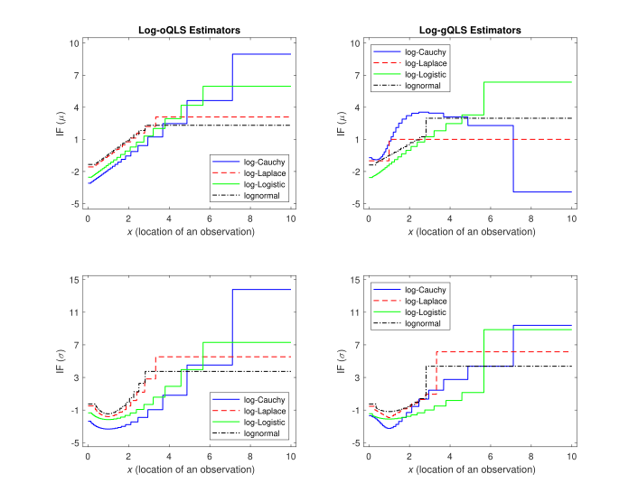
In Figure 2.1, we plot \(\text{IF} \big( x, \widehat{\pmb{\beta}}_{\text{log-oQLS}} \big)\) and \(\text{IF} \big( x, \widehat{\pmb{\beta}}_{\text{log-gQLS}} \big)\) for selected log-location-scale families using \(\mu = 0\) and \(\sigma = 1\). As suggested by illustrations in Hampel et al. (1986, chap. 2), the shapes of these IFs look like stepwise approximations of a half of the IFs of various robust estimators for location and scale parameters. But notice that there is some influence capping near \(x = 0\), the point of infinite magnitude for logarithmically transformed data. For estimation of \(\sigma\), they behave like an approximate version of an \(M\)-estimator for scale (Hampel et al. 1986, Figure 2, p. 123), with log-gQLS exhibiting a slightly sharper dip around \(x = 1\) (equivalently, \(\mu = 0 = \log (1)\)). For estimation of \(\mu\), the log-oQLS estimators act like a trimmed/winsorized mean or Huber estimator (Hampel et al. 1986, Figure 1, p. 105), and the IF of the log-gQLS estimators exhibits a variety of shapes: For lognormal and log-logistic distributions, it acts like a trimmed/winsorized mean; for log-Laplace, it behaves like a median; and for log-Cauchy, its shape resembles that of a Tukey’s biweight (Hampel et al. 1986, Figure 3, p. 151). We note in passing that the latter is a prominent example of the class of redescending \(M\)-estimators that is known to be an effective outlier rejection technique. However, the main difference between log-QLS methodology and \(M\)-estimators is this: For \(M\)-estimators, one has to “know” and specify the right shape of the IF, whereas in log-QLS estimation the IF shapes emerge naturally with no intervention from the researcher.

Figure 2.1.Influence functions of the log-oQLS and log-gQLS estimators of \(\mu\) and \(\sigma\) for log-Cauchy, log-Laplace, log-logistic, and lognormal distributions. The quantiles are selected according to (2.19) with \((a, b) = (0.15, 0.85)\) and \(k = 25\).

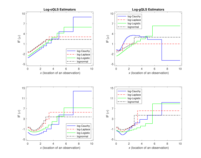
Note 2.3 Interpretation of the IF sign. If the IF is negative/positive at point \(x\), then the sample observation located at \(x\) underestimates/overestimates the corresponding parameter. For example, for all estimators in Figure 2.1, IFs are negative when \(x\) is near \(0\), leading to underestimation of \(\mu = 0\) (because \(\log x < 0\) when \(0 < x < 1\)), as well as to underestimation of \(\sigma = 1\). Interestingly, for the log-gQLS estimator of \(\mu\) under the log-Cauchy model, large values of \(x\) also lead to parameter underestimation. Finally, note that the right-most step of each IF curve remains at the same level as \(x \rightarrow \infty\) (i.e., there are no more jumps), which implies that a moderately large observation (e.g., \(x=10\)) and a huge one (e.g., \(x=10^{10}\)) have the same effect on the estimator. \(\Box\)

Note 2.4 Other roles of \(a\) and \(b\). In addition to robustness considerations, the quantile confidence levels \(a\) and \(b\) can be chosen to zoom in certain parts of the sample. This may be required by a modeling problem. For example, the choice \(a=0.01\) and \(b=0.99\) results in a log-QLS estimator that is based on almost the entire range of the sample. Such an estimator acts on data like MLE. In insurance applications, however, one is often interested in estimators that capture the upper tail well. If the tail is viewed as top 50% of the distribution, then \(a=0.50\) and \(b=0.99\) is a reasonable choice. If the tail is interpreted as top 20% of the distribution, then \(a=0.80\) and \(b=0.99\) will do the job. \(\Box\)

2.2.3. Relative efficiency and quantile selection

For the log-location-scale family of Section 2.1.1, the standard regularity conditions on \(F_{\mu, \sigma}\) are met (see, for example, Serfling 2002a, Section 4.2.2), and thus the MLE of \(\beta = (\mu, \sigma)'\) satisfies:

\[ \widehat{\pmb{\beta}}_{\mathrm{MLE}} \text { is } \mathcal{A N}\left(\pmb{\beta}, \frac{\sigma^2}{n} \mathbf{I}_*^{-1}\right), \]

where \(\mathbf{I_*}\) is the Fisher information matrix (see Table 2.1). Since MLE is the most efficient \({\cal AN}\) estimator, its performance can be used as a benchmark for the log-oQLS and log-gQLS estimators of \(\beta\). In particular, we employ the ratio of the generalized variances raised to the power \(1/m\), where \(m\) is the dimension of the parameter vector, as the asymptotic relative efficiency (ARE) criterion (Serfling 2002a, Section 4.1). For the log-location-scale family, \(m=2\) and thus we have:

\[\small{ \begin{aligned} &\text{ARE} \, \big( \text{log-oQLS}, \, \text{MLE} \big) \\&= \left( \frac{\text{det} \left[ \dfrac{\sigma^2}{n} \, \mathbf I_*^{-1} \right]} {\text{det} \left[ \dfrac{\sigma^2}{n} \, (\mathbf{X' X})^{-1} \mathbf{X'} \pmb{\Sigma_*} \mathbf{X} (\mathbf{X' X})^{-1} \right]} \right)^{1/2} \nonumber \\[1.5ex] & = \left( \frac{\text{det} \left[ \mathbf I_*^{-1} \right]} {\text{det} \big[ (\mathbf{X' X})^{-1} \mathbf{X'} \pmb{\Sigma_*} \mathbf{X} (\mathbf{X' X})^{-1} \big]} \right)^{1/2} \end{aligned} \tag{2.17}}\]

and

\[\small{\begin{aligned} &\text{ARE} \, \big( \text{log-gQLS}, \, \text{MLE} \big) \\& = \left( \frac{\text{det} \left[ \dfrac{\sigma^2}{n} \, \mathbf I_*^{-1} \right]} {\text{det} \left[ \dfrac{\sigma^2}{n} \, ( \mathbf{X'} \pmb{\Sigma^{-1}_*} \mathbf{X} )^{-1} \right]} \right)^{1/2} \nonumber \\[1.5ex] & = \left( \frac{\text{det} \left[ \mathbf I_*^{-1} \right]} {\text{det} \big[ ( \mathbf{X'} \pmb{\Sigma^{-1}_*} \mathbf{X} )^{-1} \big]} \right)^{1/2} , \end{aligned} \tag{2.18}}\]

where “det” stands for the determinant of a square matrix.

Formulas (2.17) and (2.18) match the ARE formulas for location-scale distributions, and they depend on \(k\) and how the levels \(p_1, \ldots, p_k\) are chosen. For example, by choosing \(k=2\), one could construct a percentile-matching estimator (Klugman et al. 2012, Section 13.1), which is robust but not efficient. Conversely, Adjieteh and Brazauskas (2025, Section 3.3) fixed \(p_1 = a > 0\) and \(p_{25} = b < 1\), used the uniform spacing of \(p_2, \ldots, p_{24}\) over \([a,b]\), and showed that the gQLS approach is more efficient than oQLS while offering the same degrees of robustness. Here we check whether other quantile-spacing designs can further improve the gQLS estimators’ efficiency. Thus, starting with fixed \(0 < a = p_1 < p_k = b < 1\), we consider the following strategies:

1. Uniformly-spaced probability levels \(a < p_2 < \cdots < p_{k-1} < b\): \[\small{\begin{align}p_i &= a + \frac{i-1}{k-1} (b-a), \\ i &= 1, \ldots, k.\end{align}\tag{2.19}}\] This is a distribution-free method.

2. Uniformly-spaced quantiles \(F_*^{-1}(a) < F_*^{-1}(p_2) < \cdots < F_*^{-1}(p_{k-1}) < F_*^{-1}(b)\): \[\scriptsize{\begin{align}p_i &= F_* \left( F_*^{-1}(a) + \frac{i-1}{k-1} \Big[ F_*^{-1}(b) - F_*^{-1}(a) \Big] \right), \\ i &= 1, \ldots, k.\end{align}\tag{2.20}}\] This is a distribution-dependent method.

3. Optimal \(a < p_2 < \cdots < p_{k-1} < b\). Optimal \(p_i\)’s are selected by numerically maximizing (2.18): \[\scriptsize{\begin{align}&(p_2^*, \ldots, p_{k-1}^*) ~=~ \\&\quad \operatorname*{arg\,max}_{a < p_2 < \cdots \, < p_{k-1} < \, b} \text{ARE}_k \, \big( \text{log-gQLS}, \, \text{MLE} \big) , \\ &\quad k \geq 3.\end{align}\tag{2.21}}\] This is a distribution-dependent method.

The three strategies are compared in Table 2.4 for \((a, b) = (0.05, 0.95)\) and various \(k\). From the table we first notice that the uniform spacing of \(p_i\)’s is optimal for log-Cauchy. For the other distributions, it seems like (2.20) selects \(p_i\)’s somewhat closer to the optimal ones. However, choosing \(k \geq 15\) makes \(\text{ARE}_k\)’s nearly identical across all strategies and for each distribution considered here. Hence, based on this analysis and some additional explorations, we conclude that uniform selection of \(p_1 < \cdots < p_k\) over \([a, b]\), with \(0 < a \leq 0.05\), \(0.95 \leq b < 1\), and \(k \geq 15\), is a simple, distribution-free design, which often yields very high AREs; for log-Cauchy, it is the optimal design. (For the simulation studies, real data examples, and illustrations of this paper, we use \(k=25\).)

Finally, note that AREs of all log-gQLS estimators in this study are very high (\(> 0.90\) when \(k \geq 15\)), which is remarkable. To put this in perspective, consider the situation where \(n=1,000\) data points are observed and a log-location-scale loss model must be fitted to the data at hand. While MLE would require all 1,000 points to be explicitly included in its formulas, the log-gQLS estimator would rely on only 25 (or fewer) strategically selected points, yet achieve almost identical standard errors and offer performance protection against data contamination and model misspecification.

2.3. Goodness of fit

For location-scale families, Adjieteh and Brazauskas (2025) constructed two goodness-of-fit tests using the \(\widehat{\pmb{\beta}}_{\text{gQLS}}\) estimator, which is more efficient than \(\widehat{\pmb{\beta}}_{\text{oQLS}}\). The first test was based on a quadratic form in model residuals (which are defined as sample quantiles, i.e., those that were used in estimation of \(\beta\), minus model-estimated quantiles) and was called “in-sample validation.” The main advantage of this test is that its distributional properties are analytically tractable and hence \(p\) values can be easily computed. Conversely, when \(a\) and \(1-b\) are increased, this test shrinks the range of quantiles that are used to validate the model. Thus, subsequent comparisons of two model fits with different choices of \(a\) and \(b\) are not fair. Indeed, one can achieve a nearly perfect fit by choosing both \(a\) and \(b\) (\(a < b\)) around 0.50 and thus always win the “goodness-of-fit competition” against the less extreme choices. To alleviate this problem, the second test proposed by the same authors was based on a combination of the model residuals and additional sample quantiles (the ones that had not been used for parameter estimation). It was called “out-of-sample validation.” In this paper, we modify the second test to make it workable for log-location-scale families.

To test the hypotheses

\[\small{ \left\{ \begin{array}{cl} H_0: & X_1, \ldots, X_n \text{ were generated by a log-location-scale family } F \\ H_A: & X_1, \ldots, X_n \text{ were not generated by } F, \\ \end{array} \right.}\]

the following procedure can be used.

1. Select a model-validation set of sample log-quantiles: \(\mathbf{Y}_{\text{out}} = \left( \log \widehat{F}^{-1}(p_1^{\text{out}}), \ldots, \log \widehat{F}^{-1}(p_r^{\text{out}}) \right)'\), where \(p_1^{\text{out}}, \ldots, p_r^{\text{out}}\) can be all different from or partially overlapping with \(p_1, \ldots, p_k\) (recall that \(p_1, \ldots, p_k\) were used for parameter estimation).

2. Using the linear regression model (2.13), predict the values of \(\left( \log F^{-1}(p_1^{\text{out}}), \ldots, \log F^{-1}(p_r^{\text{out}}) \right)'\) with \(\mathbf{X_{\text{out}}} \widehat{\pmb{\beta}}_{\text{log-gQLS}}\), where \[\mathbf{X}_{\text{out}} ~=~ \begin{bmatrix} 1 & \cdot & \cdot & \cdot & 1 \\[1ex] F_*^{-1}(p_1^{\text{out}}) & \cdot & \cdot & \cdot & F_*^{-1}(p_r^{\text{out}}) \\ \end{bmatrix}'\] and \(\widehat{\pmb{\beta}}_{\text{log-gQLS}} = (\widehat{\mu}_{\text{log-gQLS}},\widehat{\sigma}_{\text{log-gQLS}})'\) is based on \(\mathbf{Y} = \left( \log \widehat{F}^{-1}(p_1), \ldots, \log \widehat{F}^{-1}(p_k) \right)'\).

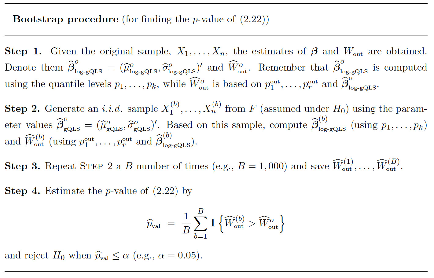
3. Construct the following test statistic out of studentized residuals: \[\small{\begin{align}W_{\text{out}} &= \frac{n}{\widehat{\sigma}^2_{\text{log-gQLS}}} \left( \mathbf{Y}_{\text{out}} - \mathbf{X}_{\text{out}} \widehat{\pmb{\beta}}_{\text{log-gQLS}} \right)' \\&\quad \pmb{\Sigma_{\text{out}}^{-1}} \left( \mathbf{Y}_{\text{out}} - \mathbf{X}_{\text{out}} \widehat{\pmb{\beta}}_{\text{log-gQLS}} \right),\end{align}\tag{2.22}}\] where the elements of \(\pmb{\Sigma_{\text{out}}}\) are given by \(\sigma_{ij}^{\text{out}} = \frac{\min \{ p_i^{\text{out}} , \, p_j^{\text{out}} \} \, - \, p_i^{\text{out}} p_j^{\text{out}} } {f_*(F_*^{-1}(p_i^{\text{out}})) f_*(F_*^{-1}(p_j^{\text{out}}))}\) for \(~i, j = 1, \ldots, r\).

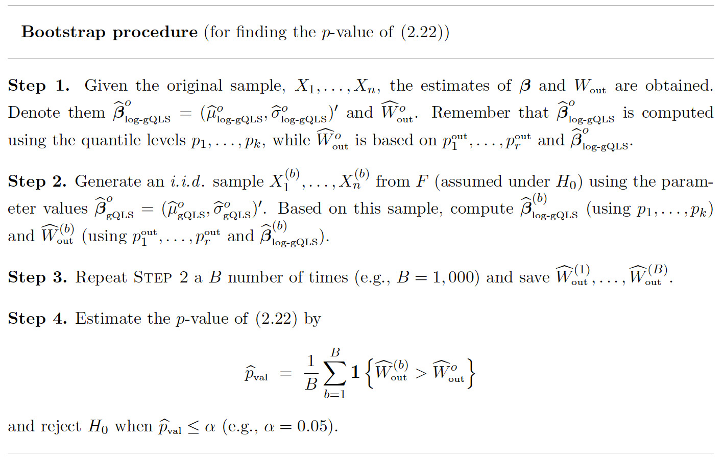
4. Estimate the \(p\)-value associated with this test statistic using the bootstrap procedure specified below. (We note in passing that theoretical treatment of the distribution of \(W_{\text{out}}\) is an ongoing challenge and is beyond the scope of the current paper.)

2.4. Pareto and Weibull

Pareto \(I\) and Weibull are two of the most popular distributions for modeling claim severity. According to the inventory of continuous loss distributions (Klugman et al. 2012, Appendix A), their pdf, cdf, and qf are parameterized as follows. For Pareto \(I\),

\[\small{\begin{aligned} f_{\text{Pa}}(x) & = \dfrac{\alpha \theta^{\alpha}}{x^{\alpha+1}}, \qquad x > \theta, \nonumber \\[1ex] F_{\text{Pa}}(x) & = 1 - (\theta/x)^{\alpha}, \qquad x \geq \theta, \nonumber \\[1ex] F^{-1}_{\text{Pa}}(u) & = \theta (1-u)^{-1/\alpha}, \qquad 0 < u < 1. \end{aligned} \tag{2.23}}\]

And for Weibull,

\[\small{\begin{aligned} f_{\text{We}}(x) & = \dfrac{\tau (x/\theta)^{\tau} e^{-(x/\theta)^{\tau}}}{x}, \qquad x > 0, \nonumber \\[1ex] F_{\text{We}}(x) & = 1 - e^{-(x/\theta)^{\tau}}, \qquad x \geq 0, \nonumber \\[1ex] F^{-1}_{\text{We}}(u) & = \theta \big( - \log (1-u) \big)^{1/\tau}, \qquad 0 < u < 1. \end{aligned} \tag{2.24}}\]

It is clear from (2.23) and (2.24) that the logarithmic transformation of \(F^{-1}\) converts Pareto \(I\) and Weibull to two-parameter exponential and Gumbel (minimum), respectively, with: \(\mu = \log \theta\), \(\sigma = 1/\alpha\) (Pareto \(I\)) and \(\mu = \log \theta\), \(\sigma = 1/\tau\) (Weibull). However, two-parameter exponential and Gumbel are skewed location-scale distributions, thus making Pareto \(I\) and Weibull log-skewed location-scale families. Therefore, statistical inference for \(\theta\), \(\alpha\), and \(\tau\) requires a bit more work than what was presented in Section 2.1.3. That is, after finding the log-oQLS and log-gQLS estimators of \(\mu\) and \(\sigma\), parameters \(\theta\), \(\alpha\), and \(\tau\) are then estimated from the expressions \(\theta = e^{\mu}\), \(\alpha = 1/\sigma\), and \(\tau = 1/\sigma\), respectively. And, to specify the \({\cal AN}\) distributions of such estimators, an additional application of the delta method is necessary. The following examples supply the missing details of this discussion.

Example 2.5 Let \(X_1, \ldots, X_n\) be i.i.d. random variables from \(\text{Pareto} \, I \, (\theta, \alpha)\) with pdf and qf parameterized as in (2.23). Suppose log-oQLS and log-gQLS of \(\mu\) and \(\sigma\) have been computed according to (2.11) and (2.12), respectively. Then, their \({\cal AN}\) distributions follow (2.14) and (2.15), respectively. Since \(\theta = e^{\mu}\) and \(\alpha = 1/\sigma\), the Jacobian of such transformations is given by

\[\mathbf{D} ~=~ \begin{bmatrix} \frac{\partial \theta}{\partial \mu} & \frac{\partial \theta}{\partial \sigma} \\[1ex] \frac{\partial \alpha}{\partial \mu} & \frac{\partial \alpha}{\partial \sigma} \end{bmatrix} ~=~ \begin{bmatrix} e^{\mu} & 0 \\[1ex] 0 & -\frac{1}{\sigma^2} \end{bmatrix} ~=~ \begin{bmatrix} \theta & 0 \\[1ex] 0 & -\alpha^2 \end{bmatrix} .\]

Therefore, it follows from the delta method that \(\left( \widehat{\theta}_{\text{log-oQLS}}, \, \widehat{\alpha}_{\text{log-oQLS}} \right)' ~=~ \left( e^{\widehat{\mu}_{\text{log-oQLS}}}, \, \frac{1}{\widehat{\sigma}_{\text{log-oQLS}}} \right)'\) is \({\cal AN}\) with the mean vector \((\theta, \alpha)\) and \(2 \times 2\) covariance-variance matrix

\[\small{ \begin{align} &\frac{\sigma^2}{n} \, \mathbf{D} \Big[ (\mathbf{X' X})^{-1} \mathbf{X'} \pmb{\Sigma_*} \mathbf{X} (\mathbf{X' X})^{-1} \Big] \mathbf{D'} \\&~=~ \frac{1}{n} \, \begin{bmatrix} \theta/\alpha & 0 \\[1ex] 0 & -\alpha \end{bmatrix} \Big[ (\mathbf{X' X})^{-1} \mathbf{X'} \pmb{\Sigma_*} \mathbf{X} (\mathbf{X' X})^{-1} \Big] \begin{bmatrix} \theta/\alpha & 0 \\[1ex] 0 & -\alpha \end{bmatrix} . \end{align} }\]

Further, following the same steps as for log-oQLS, \(\left( \widehat{\theta}_{\text{log-gQLS}}, \, \widehat{\alpha}_{\text{log-gQLS}} \right)' ~=~ \left( e^{\widehat{\mu}_{\text{log-gQLS}}}, \, \frac{1}{\widehat{\sigma}_{\text{log-gQLS}}} \right)'\) is \({\cal AN}\) with the mean vector \((\theta, \alpha)\) and \(2 \times 2\) covariance-variance matrix

\[ \small{ \begin{align} &\frac{\sigma^2}{n} \, \mathbf{D} \Big[ (\mathbf{X'} \pmb{\Sigma_*^{-1}} \mathbf{X})^{-1} \Big] \mathbf{D'} \\&~=~ \frac{1}{n} \, \begin{bmatrix} \theta/\alpha & 0 \\[1ex] 0 & -\alpha \end{bmatrix} \Big[ (\mathbf{X'} \pmb{\Sigma_*^{-1}} \mathbf{X})^{-1} \Big] \begin{bmatrix} \theta/\alpha & 0 \\[1ex] 0 & -\alpha \end{bmatrix} . \end{align} } \]

To enable the relative efficiency comparisons, the \({\cal AN}\) distribution of MLE has to be specified. Since parameter \(\theta\) is part of the domain of the Pareto \(I\) pdf, this distribution does not satisfy the well-known regularity conditions (see Serfling 2002a, Section 4.2.2). Therefore, only the univariate case, when \(\theta\) is assumed known, can be explored. But this is a straightforward exercise, as MLE-related results are readily available (see Arnold 2015, chap. 5): \(\widehat{\alpha}_{\text{MLE}} ~=~ n \big/ \sum_{i=1}^n \log (X_i/\theta)\), the Fisher information matrix (scalar) is \(\mathbf{I} = \alpha^{-2} \mathbf{I_*} = \alpha^{-2}\), and \(\widehat{\alpha}_{\text{MLE}}\) is \({\cal AN} \left( \alpha, \, \alpha^2/n \right)\).

Also, according to Note 2.2, when \(\theta\) is assumed known, log-oQLS and log-gQLS formulas need a few modifications. In particular, the modified data vector is given by

\[ \begin{align} \mathbf{Y} &~=~ \left( \log \big( \widehat{F}^{-1}(p_1) \big) - \mu, \ldots, \, \log \big( \widehat{F}^{-1}(p_k) \big) - \mu \right)' \\&~=~ \left( \log \big( \widehat{F}^{-1}(p_1)/\theta \big), \ldots, \, \log \big( \widehat{F}^{-1}(p_k)/\theta \big) \right)', \end{align} \]

and the design matrix (vector) becomes

\[\begin{align} \mathbf{X} &~=~ \left[ F_*^{-1}(p_1), \ldots, \, F_*^{-1}(p_k) \right]' \\&~=~ \left[ -\log (1-p_1), \ldots, \, -\log (1-p_k) \right]'. \end{align}\]

Therefore,

\[\small{ \begin{align} \widehat{\alpha}_{\text{log-oQLS}} &~=~ \frac{1} { ( \mathbf{X'} \mathbf{X} )^{-1} \mathbf{X'} \mathbf{Y} } \\ &\quad\text{is} \quad {\cal AN} \left( \alpha, \, \frac{\alpha^2}{n} \, (\mathbf{X' X})^{-1} \mathbf{X'} \pmb{\Sigma_*} \mathbf{X} (\mathbf{X' X})^{-1} \right) \end{align}} \]

and

\[\small{ \begin{align} \widehat{\alpha}_{\text{log-gQLS}} &~=~ \frac{1} { ( \mathbf{X'} \pmb{\Sigma_*^{-1}} \mathbf{X} )^{-1} \mathbf{X'} \pmb{\Sigma_*^{-1}} \mathbf{Y} } \\ &\quad\text{is} \quad {\cal AN} \left( \alpha, \, \frac{\alpha^2}{n} \, (\mathbf{X'} \pmb{\Sigma_*^{-1}} \mathbf{X})^{-1} \right). \end{align}} \]

Finally, the ARE formulas are given by

\[ \begin{align} &\text{ARE} \, \big( \text{log-oQLS}, \, \text{MLE} \big) \\&~=~ \left( \frac{\text{det} \left[ \dfrac{\alpha^2}{n} \right]} {\text{det} \left[ \dfrac{\alpha^2}{n} \, \Big[ (\mathbf{X' X})^{-1} \mathbf{X'} \pmb{\Sigma_*} \mathbf{X} (\mathbf{X' X})^{-1} \Big] \right]} \right)^{1/1} \\&=~ \frac{1}{(\mathbf{X' X})^{-1} \mathbf{X'} \pmb{\Sigma_*} \mathbf{X} (\mathbf{X' X})^{-1}} \end{align} \]

and

\[ \begin{align} &\text{ARE} \, \big( \text{log-gQLS}, \, \text{MLE} \big) \\&~=~ \left( \frac{\text{det} \left[ \dfrac{\alpha^2}{n} \right]} {\text{det} \left[ \dfrac{\alpha^2}{n} \, \Big[ (\mathbf{X'} \pmb{\Sigma_*^{-1}} \mathbf{X})^{-1} \Big] \right]} \right)^{1/1} \\&=~ \frac{1}{(\mathbf{X'} \pmb{\Sigma_*^{-1}} \mathbf{X})^{-1}} \text{.} \end{align} \]

For numerical illustrations, see Table 2.5.

Example 2.6 Let \(X_1, \ldots, X_n\) be i.i.d. random variables from \(\text{Weibull} \, (\theta, \tau)\) with pdf and qf parameterized as in (2.24). Suppose log-oQLS and log-gQLS of \(\mu\) and \(\sigma\) have been computed according to (2.11) and (2.12), respectively. Then, their \({\cal AN}\) distributions follow (2.14) and (2.15), respectively. Since the transformations \(\theta = e^{\mu}\) and \(\tau = 1/\sigma\) are the same as in Example 2.5, the \({\cal AN}\) distributions of log-oQLS and log-gQLS follow immediately: \(\left( \widehat{\theta}_{\text{log-oQLS}}, \, \widehat{\tau}_{\text{log-oQLS}} \right)' ~=~ \left( e^{\widehat{\mu}_{\text{log-oQLS}}}, \, \frac{1}{\widehat{\sigma}_{\text{log-oQLS}}} \right)'\) is \({\cal AN}\) with the mean vector \((\theta, \tau)\) and \(2 \times 2\) covariance-variance matrix

\[\small{ \begin{align} &\frac{\sigma^2}{n} \, \mathbf{D} \Big[ (\mathbf{X' X})^{-1} \mathbf{X'} \pmb{\Sigma_*} \mathbf{X} (\mathbf{X' X})^{-1} \Big] \mathbf{D'} \\&~=~ \frac{1}{n} \, \begin{bmatrix} \theta/\tau & 0 \\[1ex] 0 & -\tau \end{bmatrix} \Big[ (\mathbf{X' X})^{-1} \mathbf{X'} \pmb{\Sigma_*} \mathbf{X} (\mathbf{X' X})^{-1} \Big] \begin{bmatrix} \theta/\tau & 0 \\[1ex] 0 & -\tau \end{bmatrix} \end{align}} \]

and \(\left( \widehat{\theta}_{\text{log-gQLS}}, \, \widehat{\tau}_{\text{log-gQLS}} \right)' ~=~ \left( e^{\widehat{\mu}_{\text{log-gQLS}}}, \, \frac{1}{\widehat{\sigma}_{\text{log-gQLS}}} \right)'\) is \({\cal AN}\) with mean \((\theta, \tau)\) and \(2 \times 2\) covariance-variance matrix

\[\small{ \begin{align} &\frac{\sigma^2}{n} \, \mathbf{D} \Big[ (\mathbf{X'} \pmb{\Sigma_*^{-1}} \mathbf{X})^{-1} \Big] \mathbf{D'} \\&~=~ \frac{1}{n} \, \begin{bmatrix} \theta/\tau & 0 \\[1ex] 0 & -\tau \end{bmatrix} \Big[ (\mathbf{X'} \pmb{\Sigma_*^{-1}} \mathbf{X})^{-1} \Big] \begin{bmatrix} \theta/\tau & 0 \\[1ex] 0 & -\tau \end{bmatrix} .\end{align}}\]

Further, the \({\cal AN}\) distribution of MLE can be derived by exploiting the relationship between the Weibull and Gumbel (minimum) distributions. For Gumbel (minimum), the Fisher information matrix is given by

\[\mathbf{I} ~=~ \sigma^{-2} \mathbf{I_*} ~=~ \sigma^{-2} \begin{bmatrix} 1 & 1 - \gamma \\ 1 - \gamma & \frac{\pi^2}{6} + (1-\gamma)^2 \end{bmatrix} ,\]

where \(\gamma \approx 0.57721\) is the Euler-Mascheroni constant. Then, it follows from the delta method that \(\left( \widehat{\theta}_{\text{MLE}}, \, \widehat{\tau}_{\text{MLE}} \right)' ~=~ \left( e^{\widehat{\mu}_{\text{MLE}}}, \, \frac{1}{\widehat{\sigma}_{\text{MLE}}} \right)'\) is \({\cal AN}\) with mean \((\theta, \tau)\) and \(2 \times 2\) covariance-variance matrix

\[\frac{\sigma^2}{n} \, \mathbf{D} \Big[ \mathbf{I_*^{-1}} \Big] \mathbf{D'} ~=~ \frac{1}{n} \, \begin{bmatrix} \theta/\tau & 0 \\[1ex] 0 & -\tau \end{bmatrix} \Big[ \mathbf{I_*^{-1}} \Big] \begin{bmatrix} \theta/\tau & 0 \\[1ex] 0 & -\tau \end{bmatrix} .\]

Finally, for computation of AREs, the formulas (2.17) and (2.18) still remain valid, due to the properties of the matrix determinant:

\[\small{ \begin{aligned} &\text{ARE} \, \big( \text{log-oQLS}, \, \text{MLE} \big) \\& = \left( \frac{\text{det} \left[ \dfrac{\sigma^2}{n} \, \mathbf{D} \Big[ \mathbf I_*^{-1} \Big] \mathbf{D'} \right]}{\text{det} \left[ \dfrac{\sigma^2}{n} \, \mathbf{D} \Big[ (\mathbf{X' X})^{-1} \mathbf{X'} \pmb{\Sigma_*} \mathbf{X} (\mathbf{X' X})^{-1} \Big] \mathbf{D'} \right]} \right)^{1/2} \\[1.5ex] \\& = \left( \frac{\text{det} \left[ \mathbf I_*^{-1} \right]} {\text{det} \big[ (\mathbf{X' X})^{-1} \mathbf{X'} \pmb{\Sigma_*} \mathbf{X} (\mathbf{X' X})^{-1} \big]} \right)^{1/2} \end{aligned} } \]

and

\[ \small{ \begin{align} &\text{ARE} \, \big( \text{log-gQLS}, \, \text{MLE} \big) \\&~=~ \left( \frac{\text{det} \left[ \dfrac{\sigma^2}{n} \, \mathbf{D} \Big[ \mathbf I_*^{-1} \Big] \mathbf{D'} \right]} {\text{det} \left[ \dfrac{\sigma^2}{n} \, \mathbf{D} \Big[ ( \mathbf{X'} \pmb{\Sigma^{-1}_*} \mathbf{X} )^{-1} \Big] \mathbf{D'} \right]} \right)^{1/2} \\&=~ \left( \frac{\text{det} \left[ \mathbf I_*^{-1} \right]} {\text{det} \big[ ( \mathbf{X'} \pmb{\Sigma^{-1}_*} \mathbf{X} )^{-1} \big]} \right)^{1/2} .\end{align} } \]

For numerical illustrations, see Table 2.5. \(\Box\)

Using the formulas of Examples 2.5 and 2.6, Table 2.5 provides ARE values of log-oQLS and log-gQLS for the parameters of Pareto \(I\) and Weibull distributions.

3. Synthetic data illustrations

This section conducts a simulation study with the objective of verifying and augmenting the theoretical properties established in Section 2. We start by describing the study design in Section 3.1. Then we explore how the MLE, log-oQLS, and log-gQLS estimators perform when data are “clean” and when they are contaminated by outliers (Section 3.2). To see how effective the robust estimators are in identifying outliers, we apply a few well-established outlier-labeling rules on a simulated dataset (Section 3.3). We finish the study by investigating the power of the goodness-of-fit test, based on the statistic (2.22), against several alternatives (Section 3.4).

3.1. Study design

The study design is based on the following choices.

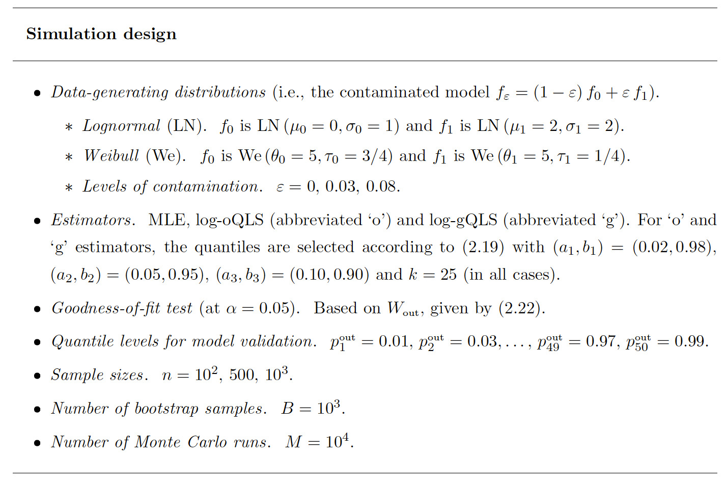
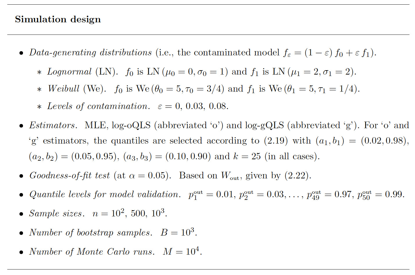
In Section 3.2, for any given distribution, we generate \(M = 10^4\) random samples of size \(n = 500\). For each sample, we estimate \(\mu\) and \(\sigma\) (or \(\theta\) and \(\tau\)) of the distribution using the MLE, log-oQLS, and log-gQLS estimators. The results are then presented using boxplots. In Section 3.3, we generate an \(8\%\) contaminated Weibull sample of size \(n = 500\). After applying several outlier-labeling rules, we evaluate their success and failure rates. In Section 3.4, the data are generated similarly as in Section 3.2, but \(n=100\) and \(1,000\). For each sample, we assume several plausible distributions and monitor the \(H_0\) rejection rates of the goodness-of-fit test (2.22). The results are summarized using tables.

3.2. Data contamination

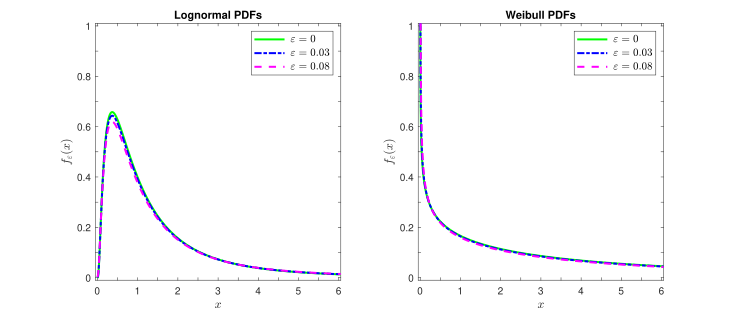
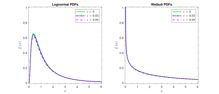
First, in Figure 3.1 we plot the clean and contaminated density functions of the lognormal and Weibull distributions. It is clear from the plots that for each model, \(f_0\), \(f_{0.03}\), and \(f_{0.08}\) are practically indistinguishable, as all three curves overlap almost everywhere, including the tails. This implies that standard diagnostic tools (e.g., histogram or quantile-quantile plot) would be unable to identify which of these models generated the data, hence, assuming \(f_0\) is a reasonable way forward. However, as our investigations demonstrate, the parameter estimates can move substantially away from their targets if data are generated by \(f_{0.03}\) or \(f_{0.08}\), instead of the assumed \(f_0\).

Figure 3.1.Lognormal and Weibull PDFs, \(f_{\varepsilon} = (1-\varepsilon) f_0 + \varepsilon f_1\), for various choices of \(\varepsilon\): \(\varepsilon = 0\) (no contamination), \(\varepsilon = 0.03\) (light contamination), \(\varepsilon = 0.08\) (moderate contamination). For the lognormal densities (LN): \(f_0\) is LN\(\, (\mu_0 = 0, \sigma_0 = 1)\) and \(f_1\) is LN\(\, (\mu_1 = 2, \sigma_1 = 2)\). For the Weibull densities (We): \(f_0\) is We\(\, (\theta_0 = 5, \tau_0 = 3/4)\) and \(f_1\) is We\(\, (\theta_1 = 5, \tau_1 = 1/4)\).

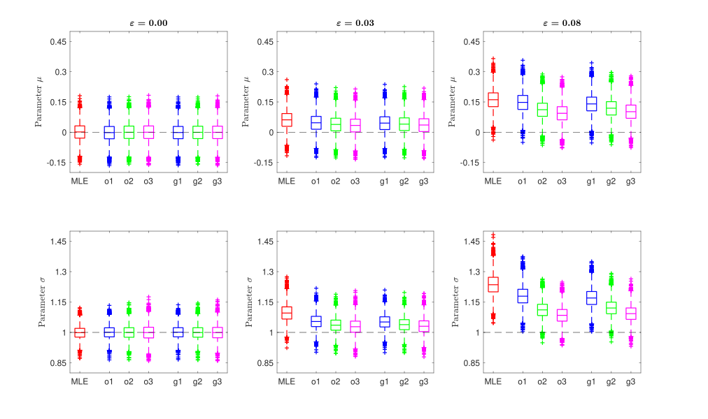
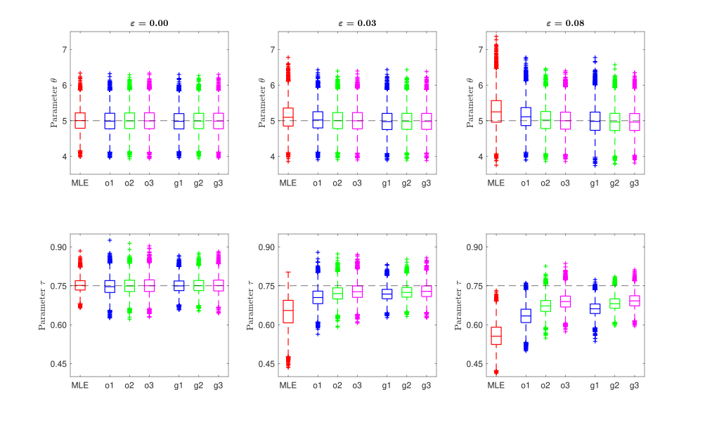
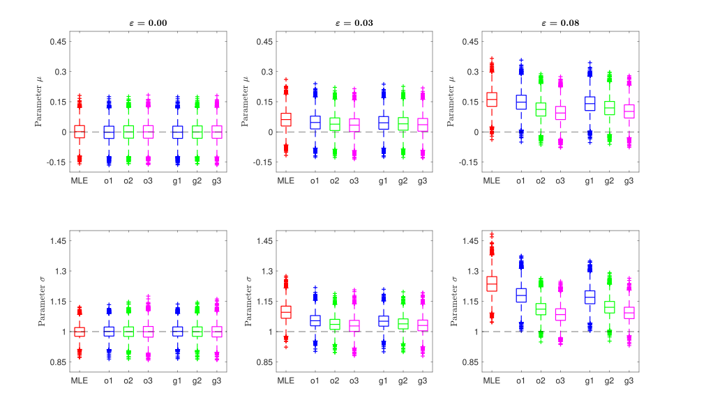
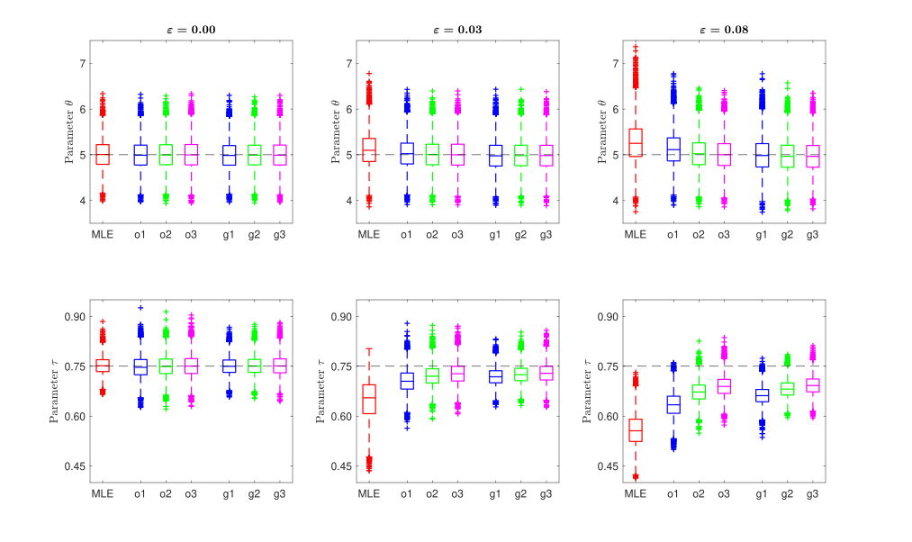
Next, we present boxplots of 10,000 estimates of \(\mu\) and \(\sigma\) (for lognormal in Figure 3.2) and \(\theta\) and \(\tau\) (for Weibull in Figure 3.3) estimators. When data are clean, we see that all estimators cluster around their respective targets, with MLE performing slightly better than log-oQLS and log-gQLS in estimating \(\sigma\) and \(\tau\). However, when data are contaminated (\(\varepsilon > 0\)), all estimators get pulled away from their targets toward the parameter values of the contaminating model \(f_1\). As expected for such scenarios, robust estimators are less affected by contamination while non-robust MLE exhibits large bias and inflated variability. Interestingly, for the Weibull distribution, only parameter \(\tau\) was contaminated, but MLE of \(\theta\) was distorted too, whereas robust log-oQLS and log-gQLS (for \(\theta\)) stayed spot on.

Figure 3.2.Lognormal\(\, (\mu, \sigma)\) distributions. Boxplots of \(\widehat{\mu}\) and \(\widehat{\sigma}\) under clean (\(\varepsilon = 0.00\)) and contaminated (\(\varepsilon = 0.03, \, 0.08\)) data scenarios, using MLE, log-oQLS/log-gQLS (‘o’/‘g’) estimators. Here \((a, b)\) is equal to \((0.02, 0.98)\) for o1/g1, \((0.05, 0.95)\) for o2/g2, and \((0.10, 0.90)\) for o3/g3.

Figure 3.3.Weibull\(\, (\theta, \tau)\) distributions. Boxplots of \(\widehat{\theta}\) and \(\widehat{\tau}\) under clean (\(\varepsilon = 0.00\)) and contaminated (\(\varepsilon = 0.03, \, 0.08\)) data scenarios, using MLE, log-oQLS/log-gQLS (‘o’/‘g’) estimators. Here \((a, b)\) is equal to \((0.02, 0.98)\) for o1/g1, \((0.05, 0.95)\) for o2/g2, and \((0.10, 0.90)\) for o3/g3.

3.3. Identification of outliers

To see how nonparametric and parametric outlier–labeling rules work, we generated 460 observations from a clean Weibull distribution (\(f_0\)) and 40 observations from a contaminating Weibull distribution (\(f_1\)). Then the combined sample of size \(n = 500\) was treated as a realization of an \(8\%\) contaminated Weibull distribution (\(f_{0.08}\)). Summary statistics for each sample are provided in Table 3.1.

Clearly, the contaminating sample is more left-skewed than the clean one because the minimum and the first two quartiles of \(f_1\) are significantly smaller than those of \(f_0\). However, \(f_1\) also has larger data points in the right tail than \(f_0\); this can be inferred from the values of \(q_3\), \(max\), \(mean\), and \(std. \, dev.\) Now, let us examine those extreme tails more carefully. In Table 3.2, 10 most extreme observations in each tail are listed for all three samples.

Looking at these data it is natural to ask: What is an outlier? We rely on the following interpretation: The data point that is smaller than the minimum or larger than the maximum observation from \(f_0\) is an outlier. For example, as shown in Table 3.2 (lines \(f_{0.08}\); the boldface entries highlight those \(f_0\) extremes that appear as extremes within the \(f_{0.08}\) sample), all observations below \(4.34 \times 10^{-3}\) and above \(54.4\) were generated by \(f_1\) and are indeed outliers. The generated sample of 500 observations has seven lower and nine upper outliers. The remaining 24 observations from \(f_1\) fall between the two extreme thresholds and assimilate with the data from \(f_0\), making it impossible to distinguish them from genuine data. Indeed, after observing the sample from \(f_{0.08}\), how can one tell that \(4.67 \times 10^{-3}\), which falls between \(4.34 \times 10^{-3}\) and \(5.06 \times 10^{-3}\), is generated by \(f_1\) and not \(f_0\)? Fortunately, the assimilated data are also harmless, i.e., their influence on the estimates of \(f_0\) parameters is similar to that of the \(f_0\) data. In view of this discussion, the quality of an outlier-labeling rule is assessed by measuring its success rates in identifying the seven lower and nine upper outliers (high rates preferred), as well as the rate of outlier-declarations in the non-extreme region. Since the latter decisions are very likely to include “false positives,” a low rate of declared outliers in this region is preferred.

Many outlier-labeling rules are available in the literature. For illustrative purposes, we selected two nonparametric and two parametric rules.

• Nonparametric rules. The classic approach of Tukey (1977, Section 2) is a very popular method, according to which outliers are those data points that fall outside the following interval: \[\small{\big[ q_1 - K \cdot (q_3-q_1); \, q_3 + K \cdot (q_3-q_1) \big],\tag{3.1}}\] where \(q_1\) and \(q_3\) denote the first and third sample quartile, respectively, and \(K=1.5\) (sometimes \(K=3\) is used). The rule (3.1) works quite well for symmetric distributions. To make it better suited for asymmetrically distributed data, Kimber (1990) proposed the following modification: \[\small{\big[ q_1 - K \cdot (q_2-q_1); \, q_3 + K \cdot (q_3-q_2) \big],\tag{3.2}}\] where \(K=1.5\) and \(q_2\) is the sample median.

• Parametric rules. The parametric approach of Banerjee and Iglewicz (2007) is designed for right-skewed distributions and focuses only on the upper outliers. It starts with the right end-point of (3.1) and replaces \(q_1\) and \(q_3\) with their respective parametric estimates, \(\widehat{q}_1 = \widehat{F}^{-1}(1/4)\) and \(\widehat{q}_3 = \widehat{F}^{-1}(3/4)\). It also uses the distribution of the largest order statistic, \(X_{(n)}\), to estimate the number of the interquartile steps \(\widehat{K} = \frac{ \widehat{F}^{-1}((1-\alpha)^{1/n}) - \widehat{q}_3}{\widehat{q}_3-\widehat{q}_1}\). This, in turn, transforms (3.1) into: \[\scriptsize{\big( -\infty; \, \widehat{q}_3 + \widehat{K} \cdot (\widehat{q}_3 - \widehat{q}_1) \big] ~=~ \big( -\infty; \, \widehat{F}^{-1} \big( (1-\alpha)^{1/n} \big) \big],\tag{3.3}}\]

where, depending upon the context, \(-\infty\) can be replaced by 0 or some other finite (known) lower bound. The term \(F^{-1} \big( (1-\alpha)^{1/n} \big)\) is derived by solving \(\alpha = \pmb{P} \big[ X_{(n)} > t \big] = 1 - [ F(t) ]^n\) for \(t\). Note that this outlier-screening rule is dependent on the sample size \(n\), making it more flexible than the nonparametric rules (3.1) and (3.2). Further, as the results of Section 3.2 demonstrate, for asymmetric distributions, the lower outliers can be as damaging to parameter estimators as are the upper outliers. Therefore, we propose to supplement the outlier-labeling rule (3.3) with an analogously designed lower bound: \[\small{\begin{align}&\big[ \widehat{q}_1 - \widehat{K}_1 \cdot (\widehat{q}_3 - \widehat{q}_1); \, \widehat{q}_3 + \widehat{K}_2 \cdot (\widehat{q}_3 - \widehat{q}_1) \big] \\&~=~ \big[ \widehat{F}^{-1} \big( 1-(1-\alpha/2)^{1/n} \big); \, \widehat{F}^{-1} \big( (1-\alpha/2)^{1/n} \big) \big],\end{align}\tag{3.4}}\] where \(\widehat{K}_1 = \frac{ \widehat{q}_1 - \widehat{F}^{-1}(1- (1-\alpha/2)^{1/n})} {\widehat{q}_3-\widehat{q}_1}\) and \(\widehat{K}_2 = \frac{ \widehat{F}^{-1}((1-\alpha/2)^{1/n}) - \widehat{q}_3} {\widehat{q}_3-\widehat{q}_1}\), and the term \(F^{-1} \big( 1-(1-\alpha/2)^{1/n} \big)\) is derived by solving \(\alpha/2 = \pmb{P} \big[ X_{(1)} \leq t \big] = 1 - [ 1 - F(t)) ]^n\) for \(t\).

Outcomes from implementing the outlier-labeling rules (3.1)–(3.4) on the 8% contaminated Weibull data (see Tables 3.1 and 3.2) are presented in Table 3.3, where we report the proportions of declared outliers in three distinct intervals: \([0; \, 4.34 \cdot 10^{-3}]\) (lower outliers), \((4.34 \cdot 10^{-3}; \, 54.4)\) (non-extreme data), and \((54.4; \, \infty)\) (upper outliers). Also, since the data are simulated from a fully specified distribution, the true values of parameters of \(f_0\) are known. Therefore, we can apply (3.3) and (3.4) with \(\theta\) and \(\tau\) estimated by MLE, log-oQLS, and log-gQLS and compare those decisions with the decision based on \(\theta_0 = 5, \, \tau_0 = 3/4\) (this will be called an “oracle decision”).

Several observations can be made from this exercise. First, (3.1)–(3.3) work poorly in identifying lower outliers, as expected. Second, the nonparametric rules (3.1) and (3.2) successfully identify all upper outliers, but that comes at the expense of declaring many outliers in the non-extreme region. Third, (3.3) and (3.4) handle the non-extreme region well. MLE-based decisions are inferior to those based on log-oQLS and log-gQLS. For Banerjee–Iglewicz rule (3.4), performances of the robust log-oQLS and log-gQLS rules get reasonably close to that of the oracle decision.

Of course, these observations are based on only one sample and thus can be coincidental. To make the analysis more reliable, we repeated the exercise on \(M=10^4\) samples of size \(n=500\). We also broadened the study by considering two distributions: 8% contaminated Weibull and 8% contaminated lognormal. The results are summarized in Table 3.4. Overall, the conclusions stated above do not change. However, among \(M=10^4\) samples, some generated either no lower or upper outliers—i.e., they were “clean” in at least one tail. Weibull had 329 such samples, and lognormal had 7,574. These were excluded from further computations. Hence, the reported outlier detection rates are valid for the samples that actually contained outliers in both tails.

3.4. Goodness of fit

The next study evaluated the power properties of the goodness-of-fit test (2.22) under several alternatives. The results are presented in Table 3.5. The following conclusions emerge from the table.

First, the test is correctly calibrated because for both distributions and for all choices of \((a, b)\) and all sample sizes, it rejects the null hypothesis (i.e., when \(f_{\varepsilon} = f_0\)) \(5\%\) of the time, which agrees with its level of significance (\(\alpha = 0.05\)). Second, under the contaminated data scenarios (i.e., when \(f_{\varepsilon} \ne f_0\)), the rejection rates increase and approach 1 as \(n \rightarrow 1,000\). This happens quite quickly for \(f_{0.08}\). Third, performance of the test in the \(f_{0.03}\) case of Weibull was fairly steady, with rejection rates fluctuating around 0.20. And for the lognormal distribution, the test starts slowly at \(n=100\), but then its performance improves rapidly. Finally, for both distributions and under all \(\varepsilon > 0\) and \(n\), higher values of \(a = 1-b\) lead to slightly higher rejection rates until they reach 1.

4. Real data examples

To illustrate how our proposed estimators, outlier-labeling rules, and the goodness-of-fit test work on real data, we used two datasets: the daily stock returns of Google for 2020 to 2023 (Section 4.1) and the normalized losses of the most damaging hurricanes in the United States from 1900 to 2022 (Section 4.2).

4.1. Google returns

We start by analyzing the daily stock returns of Alphabet Inc., the parent company of Google, for the period from January 2, 2020, to December 29, 2023. The stock prices are available at the Yahoo! Finance website (https://finance.yahoo.com/quote/GOOG/). The daily returns are computed by taking the ratio of the closing over the opening price. Table 4.1 summarizes key statistics for the log-transformed data.

Although not presented here, the histogram of the log-data revealed that a symmetric and (roughly) bell-shaped distribution might be a suitable candidate for the dataset at hand. Therefore, log-Cauchy, log-Laplace, log-logistic, and lognormal distributions were fitted to the daily returns using log-gQLS. To determine what levels of \(a\) and \(b\) are appropriate in this case, we employed the nonparametric outlier-labeling rules of Section 3.3. For Tukey (3.1), the screening interval is [-0.037; 0.039], which implies 12 lower and 11 upper outliers (of \(n = 1,006\) observations). This is equivalent to \(1.2\%\) lower and \(1.1\%\) upper contamination. For Kimber (3.2), the screening interval is [-0.023; 0.025], which declares 64 lower and 55 upper outliers. Or, equivalently, \(6.4\%\) lower and \(5.5\%\) upper contamination. Given that the two methods disagree on the levels of contamination, we selected \(a = 1-b = 0.02, \, 0.05, \, 0.10\). This mixed selection of \(a\) and \(b\) will show us if it has any material effect on further analysis. Note that all these choices are safe according to (3.1), but they offer varying levels of safety according to (3.2).

Next, model fits are formally validated using the goodness-of-fit test (2.22), for which the quantile levels (for model validation) are: \(p_1^{\text{out}} = 0.01, \, p_2^{\text{out}} = 0.03, \ldots, \, p_{49}^{\text{out}} = 0.97, \, p_{50}^{\text{out}} = 0.99\). The findings of this analysis are summarized in Table 4.2. It is clear from the table that the log-logistic distribution provides the best fit for this dataset, as its \(p\)-values are significantly greater than \(0.10\) for all three log-gQLS estimators. The log-Laplace model is borderline acceptable, with its \(p\)-values ranging between 0.06 and 0.11. The log-Cauchy and lognormal distributions are strongly rejected by the test (2.22). Also, the choice of proportions \(a\) and \(b\) has negligible effect on the goodness-of-fit of all models.

Further, as the findings of Section 3.3 suggest, the nonparametric outlier-labeling rules have a tendency to declare too many outliers. Some of those declarations are likely to be false positives. Thus, equipped with the conclusions of Table 4.2, we identified outliers using the model-based approach of Banerjee-Iglewicz (3.4). Since the log-logistic and log-Laplace models offer the best fits, they were used to identify outliers. The lognormal distribution was also included in this analysis because it plays a prominent role in many financial risk management applications. To better understand the importance of parameter estimation methods, these models are fitted using MLE, log-oQLS, and log-gQLS estimators. The results of this analysis are summarized in Table 4.3.

As is evident from Tables 4.2 and 4.3, the log-Laplace and log-logistic distributions fit this dataset well and therefore are able to accommodate the numerous nonparametrically identified outliers, 64 lower and 55 upper according to (3.4). For these models, all estimation methods (including MLE) lead to practically the same inference and decisions. Conversely, the lognormal distribution does not fit this dataset well. This seems to be due to a single upper outlier, which is successfully identified by the robust log-oQLS and log-gQLS estimators but missed by MLE.

Finally, the single upper outlier, as identified by the robustly fit lognormal model, occurred on November 30, 2022. On that day, the opening and closing prices were 95.12 and 101.45, respectively, resulting in the log-return of 0.0644. This outlier-level increase coincided with a stock rally on Wall Street after the head of the Federal Reserve said that the central bank planned to make some favorable adjustments to the interest rates. Major indexes experienced substantial but not extraordinary gains. For example, the S&P 500 rose 122.48 points, or 3.1%, to 4,080.11, and the Dow Jones Industrial Average rose 737.24 points, or 2.2%, to 34,589.77.

4.2. Hurricane damages

The second illustration uses the normalized losses from the most damaging hurricanes in the United States from 1900 to 2022, as recorded by Muller et al. (2025); see their data availability statement for the GitHub repository address where the datasets are stored. The damages were adjusted to 2022 dollars by inflation, wealth, and coastal population changes using two types of normalization: the original one proposed by Pielke and Landsea (1998), abbreviated PL22, and an alternative normalization of Collins and Lowe (2001), abbreviated CL22. The PL22-normalized damages are computed as follows:

\[D_{\text{PL22}} ~=~ D_y \times I_y \times \text{RWPC}_y \times P_{2022/y},\]

where \(D_y\) is the reported damage in landfall-year US dollars, \(I_y\) is an inflation adjustment, \(\text{RWPC}_y\) is the real wealth per capita adjustment, and \(P_{2022/y}\) is the county population adjustment. The CL22 normalization is defined by the following formula:

\[D_{\text{CL22}} ~=~ D_y \times I_y \times \text{RWHU}_y \times \text{HU}_{2022/y},\]

where \(D_y\) and \(I_y\) are defined as before, \(\text{RWHU}_y\) is the real wealth per housing unit adjustment, and \(\text{HU}_{2022/y}\) is the county housing unit adjustment. See the above-cited references for more details.

Further, it was concluded by Muller et al. (2025) that “these normalized losses showed no obvious trends over time.” To check this conclusion, we split the datasets in two periods, 1900–1999 and 2000–2022, applied our model fitting and validation methodologies on the 1900–1999 period and then used the best-fitting distributions to predict tail probabilities for the 2000–2022 period. (This choice of time periods could be labeled as the 20th century versus the 21st century.) If there is indeed no trend over time, the predictions based on well-constructed models should be close to the actually observed tail probabilities in the 21st century. Table 4.4 provides summary statistics for the PL22- and CL22-normalized losses over the period 1900–1999 (\(n=32\) hurricanes; damages measured in billions of 2022 US dollars).

Preliminary diagnostics, such as histograms of damages and log-damages, showed that an approximately log-symmetric distribution might be appropriate for both datasets. Therefore, log-Cauchy, log-Gumbel (Weibull), log-Laplace, log-logistic, and lognormal distributions were fitted to these data using log-gQLS. Also, the nonparametric outlier-labeling tests yielded between three and five upper outliers of \(n=32\) observations (equivalently, between 9.4% and 15.6% upper contamination). Specifically, Tukey (3.1) outlier-screening intervals are [-47.9; 130.9] (for PL22) and [-39.0; 120.2] (for CL22), and Kimber (3.2) intervals are [-15.4; 96.3] (for PL22) and [-3.7; 95.9] (for CL22). Since \(n=32\) is not large, the proportions \(a\) and \(b\) change quite a bit due to inclusion or exclusion of a single sample point. Therefore, we selected \((a, b) = (0.10, 0.90)\), which is a more conservative choice for the lower tail but in the range of the (3.1) and (3.2) recommendations for the upper tail.

Furthermore, Table 4.5 provides estimates of the parameters and results of the goodness-of-fit test (2.22) for the selected distributions. For model estimation, we chose \(k=15\), and for model validation, we chose \(m=15\) with the quantile levels \(p_1^{\text{out}} = 0.050, \, p_2^{\text{out}} = 0.114, \ldots, \, p_{14}^{\text{out}} = 0.886, \, p_{15}^{\text{out}} = 0.950\). Clearly (although perhaps surprisingly), the results in the table suggest that all log-gQLS-estimated models fit both datasets well, with their respective \(p\)-values substantially exceeding 0.10. Therefore, as one would expect, Banerjee-Iglewicz (3.4) identifies zero model-specific outliers in each case. Thus, according to these log-location-scale distributions, both datasets are “clean.”

The final step in this analysis was to examine the “no trends” conclusion. Using 1900–1999 data and the fitted models, we predicted the probability that the normalized damage of a hurricane happening from 2000 to 2022 exceeds a certain (high) threshold. For context, recall that during the first two decades of this century, the United States experienced some devastating hurricanes.

• Hurricane Katrina (2005). It was Category 5 at peak and 3 at landfall in Louisiana, with reported damages of \(\$125\) billion (2005 dollars) and \(1,392\) deaths (with 652 missing). Katrina devastated New Orleans due to levee failures. It is considered one of the costliest natural disasters in US history. After normalization, its damages are \(D_{\text{PL22}} = \$226.21\) and \(D_{\text{CL22}} = \$234.11\) billion.

• Hurricane Harvey (2017). It was Category 4 at landfall in Texas, with reported damages of \(\$125\) billion (2017 dollars) and 107 deaths. Harvey brought very heavy rainfall (up to 60 inches in some areas) and caused massive flooding in Houston. After normalization, its damages are \(D_{\text{PL22}} = \$164.70\) and \(D_{\text{CL22}} = \$161.12\) billion.

In view of the above discussion, we considered the following normalized thresholds: 50, 100, 150, and 200 billion. We also compared the model-based predictions with the simple empirical predictions. The results are summarized in Table 4.6. As shown in the table, all methods work well for \(t=50\), but performances diverge for higher \(t\). The empirical approach, the lognormal and log-logistic models, underestimate the probabilities of exceeding \(t = 100, ~150, ~200\). The log-Cauchy tends to overestimate the probabilities of extreme thresholds (see its predictions for \(t = 150\) and \(200\)). The log-Gumbel and log-Laplace distributions—fitted via log-gQLS with \(a=0.10\), \(b=0.90\), \(k=15\)—emerge as the most effective models for this task among the six approaches considered here. Also, for practically all entries in Table 4.6, the actual probabilities fall within one standard deviation of the predicted point estimate. For example: \(0.159 \pm 0.055\) (for log-Gumbel, PL22, \(t=100\)) covers the actual probability of 0.182, and \(0.031 \pm 0.031\) (for Empirical, PL22, \(t=200\)) includes 0.045. Overall, the “no trends” conclusion of Muller et al. (2025) seems reasonable, but more thorough investigations may change it.

5. Concluding remarks

This paper introduced four quantile and log-quantile least squares estimators for the parameters of log-location-scale loss models: ordinary (oQLS and log-oQLS) and generalized (gQLS and log-gQLS). While all estimators are equally robust, the ones based on log-quantiles are more efficient than the corresponding oQLS and gQLS estimators. Moreover, log-oQLS and log-gQLS are computationally inexpensive—they can be computed on a basic laptop in two to three minutes for samples containing a billion observations. In terms of the estimation accuracy, both “log” methods are consistent, but log-gQLS exhibits substantially smaller sampling errors than log-oQLS and often reaches 90% or higher relative efficiency when compared with the MLEs, which are theoretically optimal. Nonetheless, the log-oQLS estimator (being practically a simpler version of log-gQLS) may be easier to extend to more general loss models. Further, the advantages of log-oQLS and log-gQLS over MLE become obvious when the underlying distributional assumptions are violated by the presence of outliers. These results and properties have been established using theoretical derivations (when sample size \(n\) is large) and augmented by using simulations. Furthermore, we have applied these estimators to several data-screening rules and verified their effectiveness in identifying outliers. We observed that the success rates of log-oQLS- and log-gQLS-based rules are significantly higher than those based on MLE and slightly below the rates of the oracle rule (which mimics the scenario when the assumed underlying model is completely known). Similar conclusions were reached when these estimators were applied to a newly-designed goodness-of-fit test. That is, when sample size exceeds 100 observations, the test has sufficient power to detect and reject even mildly contaminated distributions. Of course, its power improves further against moderate or severe contamination levels. Finally, additional illustrations involving the proposed estimators, outlier-labeling rules, and the goodness-of-fit test were provided using the daily stock returns of Alphabet Inc. (Google) from 2020 to 2023 and the normalized losses of the most damaging hurricanes in the US from 1900 to 2022.

Acknowledgments

The authors are very appreciative of valuable suggestions, technical queries, and insightful comments provided by two anonymous referees, which helped to substantially improve the paper.