Application of Stochastic Differential Equations to Reserving in Non-Life Insurance

1. Introduction

The reserving process in non-life insurance is a critical task that ensures the financial health and stability of insurance companies. Traditional methods include the chain ladder, the Bornhuetter–Ferguson (BF; see Bornhuetter and Ferguson 1972), and the Cape Cod (see Bühlmann and Straub 1983) methods. These deterministic methods have been supplemented by stochastic models for chain ladder in Mack (1993), BF in Mack (2008), and Cape Cod in Saluz (2015). However, these stochastic models do not provide equations defining the overall shape of the reserving distribution but instead focus on the mean and standard deviation of the non-life reserves. To complement these approaches, in this article, stochastic differential equations (SDEs) are made equivalent to the chain ladder method (the Cox–Ingersoll–Ross, or CIR, model) and to the BF and Cape Cod methods (the arithmetic Brownian motion, or ABM). One benefit of the SDE approach is that it leads to closed-form models of the reserve distribution while requiring minimal additional assumptions.

This article focuses on two prominent SDE models: the CIR model and the ABM. The CIR model, introduced by Cox et al. (1985), is famous in finance for modeling interest rates, thanks to its mean-reverting properties. Its application in non-life insurance reserving comes naturally when the Mack model parameters for expected value and standard deviation (see Mack 1993) are converted into the drift and diffusion terms, respectively, of the CIR model. As for the BF and Cape Cod models, the same conversion of the Mack and Saluz model parameters for expected value and standard deviation into the respective drift and diffusion terms leads to an ABM model. Appendix D provides some introductory concepts about SDEs in general and introduces some specific types of SDEs.

By applying these models to the non-life reserving process, the article aims to demonstrate how SDEs can help to describe the overall non-life reserving distribution while making minimal a priori assumptions about the shape of this distribution. Such an understanding of the non-life reserving distribution may help practitioners refine reserve estimates and improve risk management, ultimately contributing to the financial resilience of non-life insurance companies.

2. The chain ladder and CIR models

This section, partially based on Dal Moro (2021), briefly describes the equivalence between the chain ladder model and the CIR model. It should be noted that the present article makes the equivalence to a constant elasticity of variance (CEV) model (for example, see Cox 1975) with \(\beta\) = 0.5. This special case of a CEV model is a CIR model, as shown in Cox et al. (1985).

As usual, let \(C_{l,k}\) denote the cumulative incurred claims amount of accident year l after k years of development, with \(1 \leq l\), \(k \leq I\), where I denotes the most recent accident year (Table 2.1).

Then \(C_{I-i+1,i}\) denotes the currently known claims amount of accident year I – i + 1. The basic chain ladder assumption is that there exist development factors \(f_1, ..., f_{I-1}\), such that

\[\small E\left(C_{i,k+1} | C_{i,1},...,C_{i,k} \right)=f_k C_{i,k}, 1 \leq i \leq I, 1 \leq k \leq {I-1},\tag{1}\]

where the link ratios (age-to-age factors) can be estimated as

\[\hat{f}_k = \frac{\sum_{j=1}^{I-k} C_{j,k+1}}{\sum_{j=1}^{I-k} C_{j,k}},\tag{2}\]

under the assumption that \(\left\{C_{i,1},...,C_{i,I}\right\},\left\{C_{j,1},...,C_{j,I}\right\}, i \neq j\) are independent. In this paper, \(\hat{f}_k\) will denote the estimator of the random variable \(f_k\). Mack (1993) shows that the link ratios \(\hat{f}_k\) are unbiased and uncorrelated.

As for the variance of \(C_{i,k + 1}\), Mack (1993) induced that \(Var\left(C_{i,k+1}| C_{i,1},...,C_{i,k}\right)\) (where \(Var\left(A|B\right)\) denotes the conditional variance of A, knowing B) should be proportional to \(C_{i,k}\), i.e.,

\[\small Var\left(C_{i,k+1} | C_{i,1},...,C_{i,k} \right)=C_{i,k} \sigma_k^2, 1 \leq i \leq I, 1 \leq k \leq {I-1},\tag{3}\]

where

\[\small \sigma_k^2=\frac{1}{I-k-1} \sum_{i=1}^{I-k} C_{i,k} \left( \frac{C_{i,k+1}}{C_{i,k}}-\hat{f}_k \right)^2 for \ 1 \leq k \leq I-2.\tag{4}\]

It can be shown that the estimator \(\hat{\sigma}_k^2\) is unbiased (for example, see Mack 1993).

In order to translate the properties just discussed into an SDE framework, we need to define the equivalent drift and diffusion terms so that the expected value and the standard deviation of the resulting SDE match with equations (1) and (3), respectively. For the drift term, we have

\[\small \Delta C_{i,k}= C_{i,k+1}-C_{i,k}=f_k C_{i,k} - C_{i,k} = \left(f_k - 1\right) C_{i,k},\tag{5}\]

which can be translated in continuous time as

\[d C_{i,k}= log\left(f_k \right) C_{i,k} dk.\tag{6}\]

As for the diffusion term, equation (3) provides that

\[\small Var\left(C_{i,k+1} | C_{i,1},...,C_{i,k} \right)=C_{i,k} \sigma_k^2, 1 \leq i \leq I, 1 \leq k \leq {I-1}\tag{7}\]

and

\[\implies \sigma \left(C_{i,k+1} | C_{i,1},...,C_{i,k} \right)= \sigma_k \sqrt{C_{i,k}},\tag{8}\]

where \(\sigma \left(A\right)\) denotes the standard deviation of random variable A.

As a result, the following SDE comes naturally:

\[dC_{i,k}=log \left\{f_k\right\} C_{i,k}dk + \tau_k \sqrt{C_{i,k}} dW_k,\tag{9}\]

where \(W_k\) is a Brownian motion and \(\tau_k\) is defined according to Mack (1999), who proved that

\[\small Var \left(C_{i,k+1}\right) = \sigma_k^2 C_{i,k} \left(1+\frac{C_{i,k}}{\sum_{j=1}^{n-k} C_{j,k}}\right) + \hat{f}_k^2 \text{Var}\left(C_{i,k}\right).\tag{10}\]

On the basis of equation (10), we will define \(\tau_k\) in the following paragraphs using this definition of the chain ladder volatility:

\[volCL_{i,k}^2 = \sigma_k^2 \left(1 + \frac{C_{i,k}}{\sum_{j=1}^{n-k} C_{j,k}} \right).\tag{11}\]

Equation (9) corresponds to a CIR model, which has a closed-form solution. A CIR model is given by the following SDE:

\[dr_t=\kappa(\theta-r_t)dt+\tau \sqrt{r_t}dW_t,\tag{12}\]

where

• \(r_t\) is the interest rate at time t,

• \(\kappa\) is the speed of mean reversion,

• \(\theta\) is the long-term mean level,

• \(\tau\) is the volatility, and

• \(W_t\) is a Brownian motion.

The exact solution for \(r_t\) can be expressed in terms of a noncentral chi-squared distribution. If \(r_0\) is the initial interest rate, then \(r_t\) follows:

\[r_t=\frac{\tau^2 \left(1-e^{-\kappa t}\right)}{4 \kappa} \chi_{\frac{4 \kappa \theta}{\tau^2}}^2 \left(\frac{4 \kappa r_o e^{-\kappa t}}{\tau^2 \left(1-e^{-\kappa t}\right)}\right).\tag{13}\]

In order to have a correspondence between the chain ladder model from Mack (1993) and the CIR model, we choose the following parameters:

• \(\kappa_t = - log \left\{f_t\right\}\)

• \(\theta = 0\)

• \(\tau_t^2 = \frac{volCL_{i,t}^2}{\hat{f}_t} \frac{log\left({\hat{f}_t}\right)}{\left(\hat{f}_t-1\right)}\)

Because \(r_t\) follows a noncentral chi-square distribution with zero degrees of freedom, expressed as \(\theta = 0\) (see Siegel 1979), using the above parameters, we can calculate the expected value of \(C_{i,t+1}\), knowing \(C_{i,t}\) (we just make the equivalence of \(r_t\) = \(C_{i,t}\)), as follows:

\[\small E \left(C_{i,t+1} | C_{i,t}\right) = \frac{\tau_t^2 \left(1-e^{-\kappa_t}\right)}{4 \kappa_t } E\left(\chi_0^2 \left(\frac{4 \kappa_t C_{i,t} e^{-\kappa_t}}{\tau_t^2 \left(1-e^{-\kappa_t}\right)}\right) \right)\tag{14}\]

\[\implies E \left(C_{i,t+1} | C_{i,t}\right)= f_t C_{i,t}.\tag{15}\]

Equation (15) corresponds to the expected value of the chain ladder model (see equation (1)).

In the same way, we can calculate the variance of \(C_{i,t+1}\) knowing \(C_{i,t}\) (see Appendix C for calculation details):

\[Var \left(C_{i,t+1} | C_{i,t}\right)=volCL_{i,t}^2 C_{i,t} + \hat{f}_t^2 Var \left(C_{i,t}\right).\tag{16}\]

Equation (16) corresponds to the variance of the chain ladder model (see equation (10)).

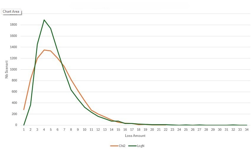
Following the above analysis, Appendix E provides a high-level comparison of a lognormal distribution versus a noncentral chi-square distribution with zero degrees of freedom. It depicts graphically how these two distributions are similar and how they are different.

As a conclusion for this section, the lognormal distribution—commonly assumed to describe the full non-life reserving distribution—does not appear to be consistent with the proposed model. The SDE framework developed here suggests that the natural analogue of the chain ladder method leads instead to a noncentral chi-square distribution with zero degrees of freedom. This distribution provides an alternative basis for estimating the quantiles of the reserving distribution. A systematic comparison of the quantile estimates produced by the lognormal and noncentral chi-square distributions represents a promising direction for future research.

3. Equivalence of the BF and Cape Cod methods to the ABM model

Having described an equivalent SDE for the chain ladder reserving model, we will now focus on an equivalent for the BF and Cape Cod reserving models.

3.1. The BF reserving model

Using the procedure outlined by Mack (2008), the stochastic model underlying the BF reserving model should be applied to incremental triangles, in contrast to the chain ladder model, which applies to cumulative triangles.

With the same notation as in the chain ladder model, let \(S_{i,k}=C_{i,k}-C_{i,k-1}\) denote the incremental claims amount (with \(C_{i,0}=0\)) and \(U_i\) the (unknown) ultimate claims amount of accident year i. Let \(\nu_i\) be the premium volume of accident year i, and let n denote the most recent accident year. Then \(R_i=U_i-C_{i,n+1-i}\) is the (unknown true) claims reserve for accident year i. Finally, let \(S_{i,n+1}=U_i-C_{i,n}\) be the estimated tail development of the claims amount after development year n.

Bornhuetter and Ferguson (1972) give the BF method to estimate \(R_i\) as follows:

\[\hat{R}_i^{BF}=\hat{U}_i\left(1-\hat{z}_{n+1-i}\right),\tag{17}\]

where \(\hat{U}_i=\nu_i \hat{q}_i\), with a prior estimate \(\hat{q}_i\) for the ultimate claims ratio \(q_i=\frac{U_i}{\nu_i}\) of accident year i, and \(\hat{z}_k \in [0;1]\) is the estimated percentage of the ultimate claims amount that is expected to be known after development year k.

In Mack (2008), the stochastic model for the BF method shares a similar structure with the chain ladder model of Mack (1993) while adequately reflecting the two fundamental differences between the two methods. The first difference concerns the nature of the reserve estimate: While the chain ladder reserve is directly proportional to the cumulative claims amount observed to date, the BF reserve is entirely independent of the known claims experience. This distinction is captured in the BF model through an additional independence assumption, which formalizes the foundational BF principle that past and future claims—that is, \(C_{i,n+1-i}\) and \(R_i^{BF}\), respectively—are independent of one another. This independence between past and future claims was indeed central to the original formulation of the BF method. The second difference follows naturally from this independence principle: Since future claims do not depend on past claims within the same accident year, it is appropriate to assume that all increments \(S_{i,k}\) belonging to the same accident year are mutually independent. This assumption, combined with the standard assumption of independence across accident years, provides the probabilistic foundation upon which the stochastic BF model is built. As a consequence, the BF stochastic model developed by Mack (2008) relies on the following assumptions related to the increments \(S_{i,k}\):

• BF1: All increments \(S_{i,k}\) are independent.

• BF2: There are unknown parameters \(x_i\), \(y_k\) such that

  • \(E\left(S_{i,k}\right)=x_i y_k\) and

  • \(y_1+\dots+y_{n+1}=1\).

• BF3: There are unknown proportionality constants \(s_k^2\) with \(Var\left(S_{i,k}\right)=x_i s_k^2\).

It is worth noting that \(x_i\) is the a priori estimate of the ultimate loss for accident year \(i\) and \(y_k\) is the incremental percentage of the ultimate loss for development period \(k\).

Using the approach of Mack (2008), we have the following with \(x_1,...,x_n\) known:

\[\hat{y}_k=\frac{\sum_{i=1}^{n+1-k} S_{i,k}}{\sum_{i=1}^{n+1-k} x_i}\tag{18}\]

is a best linear unbiased estimate of \(y_k\), and

\[\hat{s}_k^2 = \frac{1}{n-k} \sum_{i=1}^{n+1-k} \frac{\left(S_{i,k} - x_i \hat{y}_k\right)^2} {x_i}\tag{19}\]

is an unbiased estimate of \(s_k^2\).

Having estimated the parameters \(\hat{y}_k\) and \(\hat{s}_k^2\) (see Mack 2008 for details on the estimation process), we can calculate the BF claims reserve by

\[\begin{align} \hat{R}_i^{BF}=&\hat{U}_i\left(\hat{y}_{n+2-i}+...+\hat{y}_{n+1}\right)=\hat{U}_i\left(1-\hat{z}_{n+1-i}\right) \\& with \ \hat{z}_k=\left(\hat{y}_1+...+\hat{y}_k\right).\end{align}\tag{20}\]

The properties of these estimators are as follows:

• \(\hat{y}_1,..., \hat{y}_{n+1}\) are pairwise (slightly) negatively correlated, as they have to add up to unity.

• \(\hat{y}_1,..., \hat{y}_{n+1}\) and \(\hat{z}_1,..., \hat{z}_{n+1}\) are independent from \(\hat{U}_1,..., \hat{U}_n\).

• \(E\left(\hat{U}_i\right)=E\left(U_i\right)=x_i\) for \(1 \leq i \leq n\).

• \(E\left(\hat{y}_k\right)=y_k\) for \(1 \leq i \leq n+1\) and therefore \(E\left(\hat{z}_k\right)=z_k\).

• \(E\left(\hat{s}_k^2\right)=s_k^2\) for \(1 \leq i \leq n+1\).

Based on the above notations, the mean squared error of prediction of \(\hat{R}_i^{BF}\) is given as

\[\scriptsize \begin{aligned} \hat{msep}\left(\hat{R}_i^{BF}\right)=&\hat{U}_i \left(\hat{s}_{n+2-i}^2 + ... + \hat{s}_{n+1}^2\right) \\& +\left(\hat{U}_i^2+Var\left(\hat{U}_i\right)\right) Var \left(\hat{z}_{n+1-i}\right) \nonumber \\ &+Var\left(\hat{U}_i\right) \left(1-z_{n+1-i}\right)^2. \end{aligned}\tag{21}\]

As we want to apply an SDE for each development year t of accident year i, we have to split \(\hat{msep}\left(\hat{R}_i^{BF}\right)\) into its development year components. The first element of equation (21) is already split into its development year elements. For the second element of the equation, according to Mack (2008), we can do the following replacement, being on the safe side:

\[\small Var \left(\hat{z}_{n+1-i}\right)=\left(Var\left(\hat{y}_{n+2-i}\right)+...+Var\left(\hat{y}_{n+1}\right)\right).\tag{22}\]

This splits the second element of equation (21) into its development year elements. Finally, for the third element of equation (21), we have

\[\scriptsize \left(1-z_{n+1-i}\right)^2=\left(\hat{y}_{n+2-i}+...+\hat{y}_{n+1}\right)^2=\sum_{l=n+2-i}^{n+1}\hat{y}_l \left(\hat{y}_l +2 \sum_{t=l+1}^{n+1} \hat{y}_{t}\right).\tag{23}\]

As in Mack (2008), we further estimate \(Var\left(\hat{y}_{k}\right)\) as follows:

\[Var\left(\hat{y}_{k}\right)=\frac{\hat{s}_k^2}{\sum_{j=1}^{n+1-k} \hat{U}_j}.\tag{24}\]

And we also estimate \(Var\left(\hat{U}_i\right)\) with the coefficient of variation of \(\hat{U}_i\), which we denote as \(c.v.(\hat{U}_i)\). This coefficient of variation could come from pricing studies, for example. In any case, it will be an external parameter. With these elements, we can now provide the mean squared error of prediction per increment of each development year t of accident year i:

\[\scriptsize \begin{aligned} \hat{msep}^{increment}\left(\hat{R}_{i,t}^{BF}\right)=&\hat{s}_{t+1}^2 \hat{U}_i \left(1+\frac{\hat{U}_i \left(1+c.v.(\hat{U}_i)^2\right) }{\sum_{l=1}^{i-t} \hat{U}_l}\right) \nonumber \\& + \left(c.v.(\hat{U}_i)\hat{U}_i\right)^2 \left( \hat{y}_{t+1} \left(\hat{y}_{t+1}+2 \sum_{l={n+2-i}}^{t} \hat{y}_{l}\right) \right) \end{aligned}\tag{25}\]

and

\[n-i+1 \leq t \leq n \nonumber.\]

Due to the independence of the increments, the mean squared error of prediction for the cumulative claims amount of each development year t of accident year i is estimated as follows:

\[\hat{msep}^{cumul.}\left(\hat{R}_{i,t}^{BF}\right)=\sum_{n+2-i}^{t} \hat{msep}^{increment}\left(\hat{R}_{i,t}^{BF}\right).\tag{26}\]

With this latter equation, we are ready to describe an SDE for the BF model.

As a starting point, for an accident year i in development year t, the drift term and diffusion term are given by

\[\text{Drift term = }\hat{U}_i \hat{y}_t\]

and

\[\text{Diffusion term = }\sqrt{\hat{msep}^{cumul.}\left(\hat{R}_{i,t}^{BF}\right)}.\]

Neither the drift term nor the diffusion term depends on its value in the previous development year. Hence, the equivalent SDE for the BF model is simply the ABM:

\[dC_{i,t}=\hat{U}_i \hat{y}_t dt + \sqrt{\hat{msep}^{cumul.}\left(\hat{R}_{i,t}^{BF}\right)} dW_t.\tag{27}\]

The solution of this SDE is given by a normal distribution with parameters

\[C_{i,t+1}=N\left(C_{i,t} + \hat{U}_i \hat{y}_t, \hat{msep}^{cumul.}\left(\hat{R}_{i,t}^{BF}\right)\right),\tag{28}\]

where N denotes the standard normal distribution with mean \(\hat{U}_i \hat{y}_t\) and variance \(\hat{msep}^{cumul.}\left(\hat{R}_{i,t}^{BF}\right)\).

Intuitively, the practicing actuary will usually use the BF method to reduce the uncertainty of the chain ladder model, in particular for the most recent years. Under the limiting assumption of ABM, the last equation indicates that the resulting BF reserves will have a normal distribution. The resulting normal distribution is due to the independence of the increments: In a BF process, the future evolution of the claims amounts is entirely determined by its present value, and the past trajectory of the process carries no additional predictive information. In the SDE framework, such a process translates naturally into an ABM, whose fundamental property is that it is a memoryless process. In addition, this model will indeed reduce the uncertainty of the chain ladder model, as the normal distribution does not show any skewness. Hence, the probability of getting higher reserve amounts will be significantly reduced through use of the BF model.

3.2. The Cape Cod reserving model

Having looked at the BF model, we will now review the Cape Cod model. Using the same notations as above (in Bühlmann and Straub 1983), the Cape Cod predictor for the ultimate claims of accident year i, denoted \(\hat{C}_{i,n}^{CC}\), is given by

\[\hat{C}_{i,n}^{CC} = C_{i,n+1-i} + \nu_i \hat{q}\left(1-\hat{z}_{n+1-i}\right),\tag{29}\]

where \(\nu_i\) is the earned premium of accident year i and

\[\hat{q}=\frac{\sum_{i=1}^{n} C_{i,n-i}}{\sum_{i=1}^{n} \nu_i \hat{z}_{n-i}}.\tag{30}\]

Equation (30) can be interpreted as \(\hat{q}\) representing a loss ratio derived from the known triangle.

Equation (29) is essentially the same as equation (17) if we replace \(\hat{U}_i\) with \(\nu_i \hat{q}\). Therefore, the same ABM model can be applied to the Cape Cod model. And we can conclude that use of the Cape Cod model will also lead to a reserving distribution that follows a normal distribution. As for the BF model, the practicing actuary will usually use the Cape Cod model as an alternative to the BF model when the chain ladder model shows a significant uncertainty in its results. In addition, the Cape Cod model will reduce the uncertainty of the BF model’s overall ultimate claims reserve amounts.

4. Combining the CIR and ABM models

We have now established the reserving distributions resulting from use of the chain ladder model and the BF (respectively, Cape Cod) model. Usually, practicing actuaries will calculate weighted averages of these methods for the most recent accident years. The aggregation of two distributions requires knowledge about their dependency. This section will therefore examine the dependency between the chain ladder and BF (respectively, Cape Cod) model. Once this dependence is established, it will be easy to combine the two distributions using, for example, a copula or simply a correlation.

For one accident year i, we can estimate the series of future cumulative claims amounts starting from the last known claims amount, \(C_{i,n+1-i}\), for both the chain ladder and BF methods:

• Chain ladder: \(\hat{C}_{i,n-i+t+1}^{CL}=C_{i,n+1-i} \prod_{l=n+1-i}^{n-i+t} \hat{f}_l\).

• BF: \(\hat{C}_{i,n-i+t+1}^{BF}=C_{i,n+1-i} + \hat{U}_i*\left(\hat{z}_{n-i+t+1}-\hat{z}_{n+1-i}\right)\).

It is usual in the practice to use the same pattern for the chain ladder method and the BF method. In this case, we can relate \(\hat{f}_t\) and \(\hat{z}_t\) as follows:

\[\hat{z}_t=\frac{1}{\prod_{l=t}^{n} \hat{f}_l}.\tag{31}\]

Let us denote the ultimate claims amount of the chain ladder model as

\[Ult_{i}^{CL}=C_{i,n+1-i} \prod_{l=n+1-i}^{n} \hat{f}_l.\tag{32}\]

With this definition, the series of chain ladder cumulative claims amounts becomes

\[\hat{C}_{i,n-i+t+1}^{CL}=Ult_{i}^{CL} \prod_{l=n-i+t+1}^{n} \hat{f}_l = Ult_{i}^{CL} \hat{z}_{n-i+t+1}.\tag{33}\]

By construction, we have

\[C_{i,n+1-i} \approx Ult_{i}^{CL} \hat{z}_{n-i+1}.\tag{34}\]

We finally get

\[\small \hat{C}_{i,n-i+t+1}^{CL} \approx C_{i,n+1-i} + Ult_{i}^{CL} \left(\hat{z}_{n-i+t+1}-\hat{z}_{n+1-i}\right).\tag{35}\]

As a result, for one accident year i, the chain ladder and BF series of projected claims amounts follow the same pattern: \(\hat{z}_{n-i+t+1}-\hat{z}_{n+1-i}\). Thus, they are heavily correlated. This is expected, as the underlying projection models use the same projection pattern (see Dal Moro (2024) for more information on projection patterns). In conclusion, when calculating the weighted average of the noncentral chi-squared distribution (for the chain ladder model) and of the normal distribution (for the BF model), we can assume a full dependency between the two distributions.

5. Numerical examples

This section illustrates the concepts described above using two triangles (see Appendix A and Appendix B). For both triangles, projected claims values and standard deviations (according to Mack 1993, 2008) for the chain ladder and BF models are provided in Appendix A and Appendix B.

As for the SDE, for each future development year of each accident/underwriting year, we fit a CIR model to the chain ladder Mack model (expected value and standard deviation), as shown in Table 5.1.

Using equation (13), we have the following:

\[C_{i,t+1}=\frac{volCL_{i,t}^2}{4 \hat{f}_t} \chi_0^2 \left( \frac{4 \hat{f}_t C_{i,t}}{volCL_{i,t}^2} \right).\]

And for the BF model, we fit an ABM model, as shown in Table 5.2.

The solution to the equation embedded in Table 5.2 is provided in equation (28).

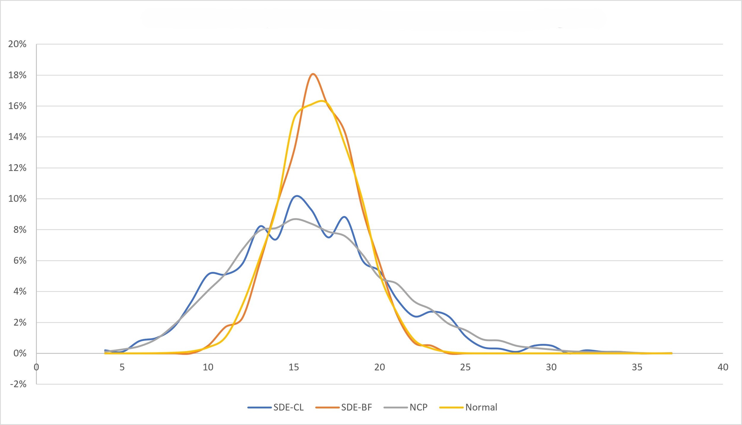
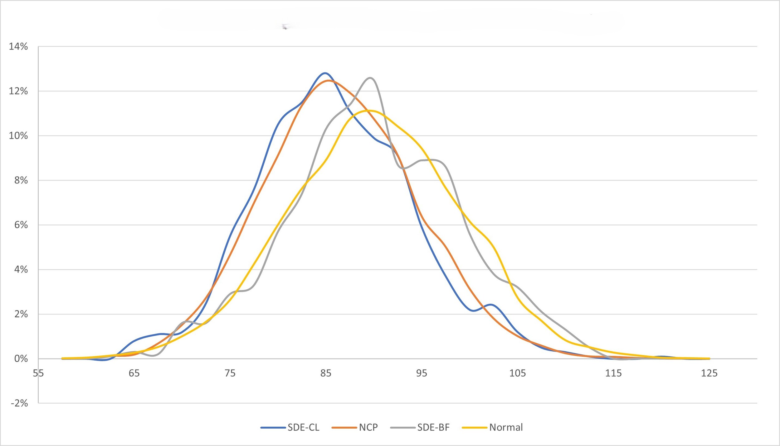
Using the package Sim.Diffproc from R and its snssde2d program,^[1] it is easy to simulate, step by step, the SDE for each accident year and each development year in the future for both the CIR model and the ABM model. In this context, 1,000 simulations were performed in R for each future development year of each accident year. Figures 5.1 and 5.2 depict two examples of the resulting simulated distributions (using the R simulations), compared with the formulaic distributions (noncentral chi-square distribution for chain ladder and normal distribution for BF).

Figure 5.1.Triangle 1—Comparison of different distributions and simulation results for accident year 8 / development year 10 of triangle 1. Note: NCP denotes the noncentral chi-square distribution with zero degrees of freedom, being the formulaic distribution of the chain ladder model. SDE-CL denotes the simulated chain ladder model using the R program. SDE-BF denotes the simulated BF model using the R program. Normal denotes the normal distribution, being the formulaic distribution of the BF model.

Figure 5.2.Triangle 2—Comparison of different distributions and simulation results for accident year 7 / development year 7 of triangle 2.

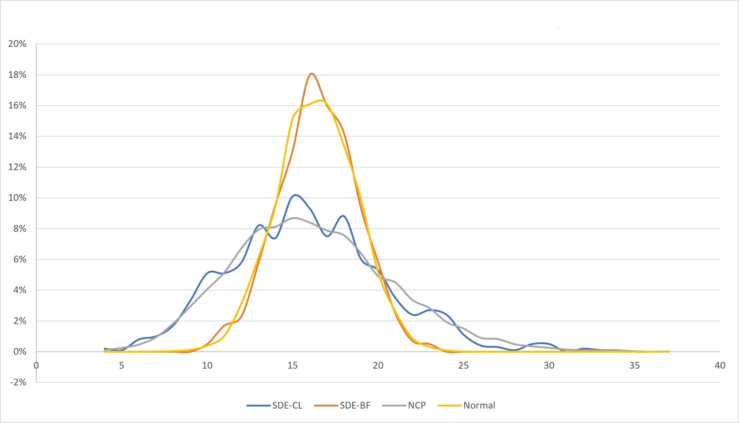
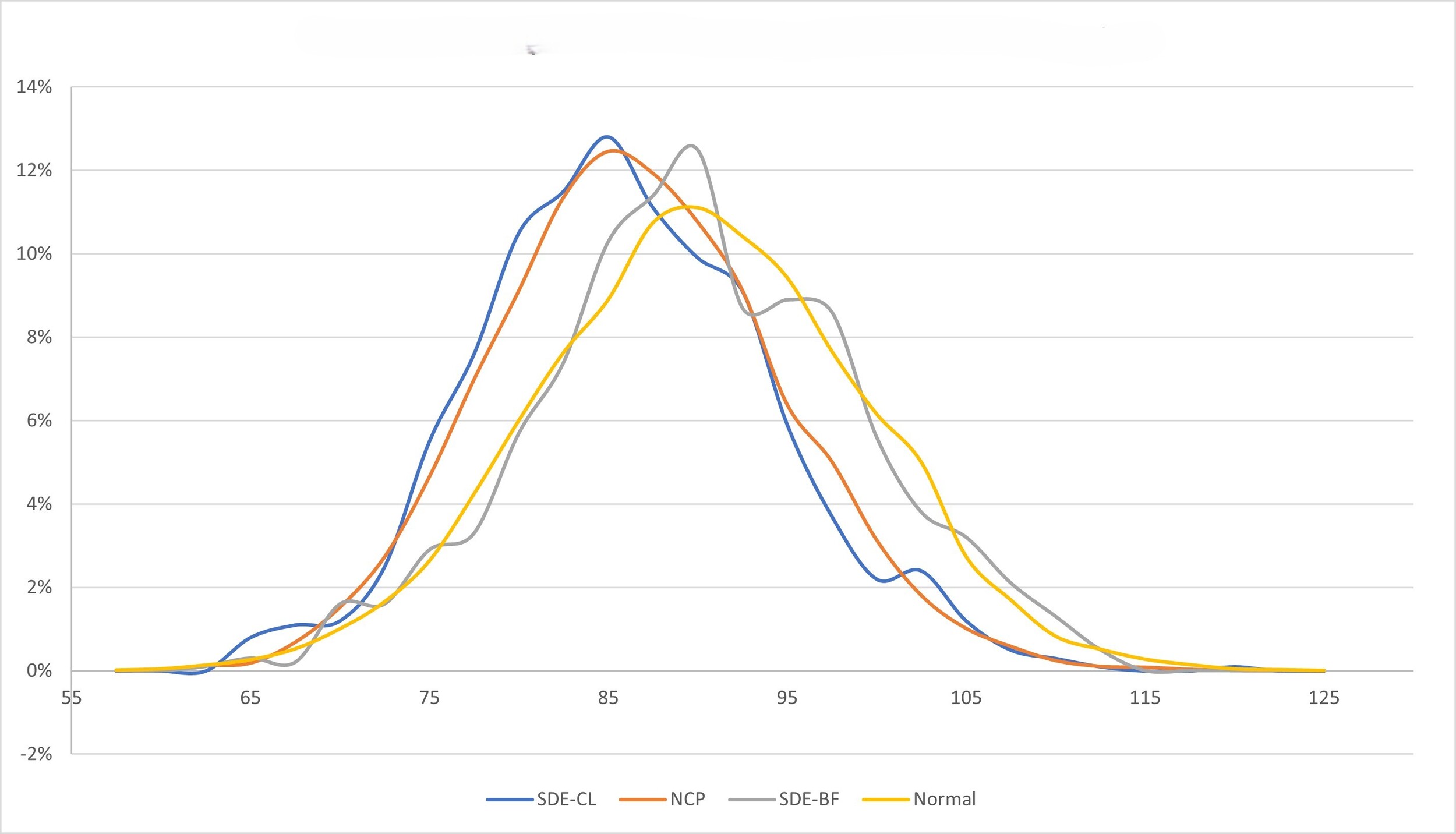
In both figures, even with only 1,000 simulations, we can see that the simulated distribution is very close to the formulaic distribution, as expected. In addition, we can see that the BF model leads to a distribution with a lower volatility and a lower skewness compared with the distribution resulting from the chain ladder model. This is also expected. These two examples show that, with minimal assumptions, it is possible to derive the shape of the non-life reserving distributions for each projected cell of a triangle.

6. Conclusion

In practice, non-life actuaries tend to use the lognormal distribution for modeling the overall shape of the non-life insurance reserve distribution, whatever the method used to project the reserves. The use of the lognormal distribution is justified by its simplicity and availability in Excel. It is also a convenient choice, as the support of the distribution is on \([0,+\infty)\), thereby avoiding negative reserve values (which is a desired feature). The lognormal distribution also differs from a normal distribution by having a positive skewness, allowing more extreme events to be included in the distribution. Despite the many desirable features of the lognormal distribution, there is no justification in the literature for using it to represent the overall non-life reserves. In this context, this article intended to examine which distribution should be chosen for the different known reserving methods, while making minimal assumptions. The use of SDE allows such a study and leads to different distributions, namely the noncentral chi-square distribution with zero degrees of freedom in the case of the chain ladder projection method and the normal distribution in the case of the Cape Cod and BF methods. The noncentral chi-square distribution with zero degrees of freedom has the same advantages as the lognormal distribution:

• The support of the distribution is also \([0,+\infty)\), thereby avoiding negative reserve values.

• It has a positive skewness.

For chain ladder, it is therefore recommended to use this distribution instead of the lognormal distribution.

As for the BF and Cape Cod methods, on the other hand, the normal distribution may feature negative reserves, but a negative reserve is likely, in practice, to remain a remote possibility, as the standard deviations should remain small. Therefore, for these methods, it is recommended to use a normal distribution to reflect the underlying dynamics of the projection methods.

Finally, the investigation presented in this article could be extended by fitting the known skewness estimators to the noncentral chi-square distributions for chain ladder and to the normal distribution for BF and Cape Cod. In the case of the noncentral chi-square distribution, it seems that there will not be a formulaic distribution, but for the BF and Cape Cod cases, a skew-normal distribution should be chosen. Such a study should be done in an upcoming article.