
1. Introduction
As underwriters of risk, insurance companies play a primary role in managing the impact of natural disasters. A report by the Intergovernmental Panel on Climate Change (2022) concludes that both the frequency and severity of natural disasters are on the rise, posing a great challenge to the sustainability of the insurance industry. Florida currently has more than 10 insurance companies placed under receivership—many as a result of property and casualty losses.[1] Some major insurers, such as State Farm, Allstate, and Farmers Insurance, are discontinuing their homeowners’ insurance businesses in certain states because they no longer consider them profitable. These facts highlight the importance of accurately modeling climate-related insurance losses to support pricing, reserving, and risk management in actuarial practice.
In traditional insurance risk analysis, frequency and severity are often modeled separately. For example, catastrophic losses are commonly modeled by a compound Poisson process, in which event arrivals and magnitudes are assumed to be mutually independent and the occurrence rate of catastrophes is a constant (see, e.g., Muermann 2008; Nowak and Romaniuk 2013; Tang and Yuan 2019). While this model setup is appealing for its mathematical tractability, it fails to capture several salient features of extreme climate events.
First, climate extremes, such as extreme precipitation, droughts, floods, and storms, typically exhibit temporal clustering behavior; that is, they often occur one after another within a short period of time. For empirical studies on the clustering of climatic events (see Villarini et al. 2010; Barton et al. 2016; Gu et al. 2016; Parente et al. 2016; Herrera-Estrada et al. 2017; Mallakpour et al. 2017). Second, the occurrence rates and severity distributions of climatic events are time-varying. For example, some extreme weather and climate events are becoming more frequent and/or intense due to climate change; see Seneviratne et al. (2023) and references therein. Moreover, in years with abnormal climate cycles, such as 2023 with El Niño, we have witnessed numerous devastating disasters, including Hurricane Idalia and the Maui wildfires, which caused tremendous economic and livelihood losses. Third, climate risks tend to compound, causing the frequency and severity of climatic events to become dependent. For example, a heatwave can decrease rainfall and impair plant growth. Without the insulation provided by plants, the heat situation is further exacerbated. This increases the likelihood of wildfires, and when they occur, they tend to be widespread. As more plants are burned and heating intensifies, the risk of future wildfires increases.
To account for these phenomena, we propose using a self-exciting peaks-over-threshold (POT) model, which integrates a self-exciting point process for frequency modeling and extreme value theory for severity modeling, to jointly model the frequency and severity of climate extremes. Within this framework, the occurrence of extreme events is modeled by a Hawkes process, whose intensity depends on past events, whereas the magnitudes of individual events are assumed to follow a generalized Pareto distribution (GPD) with a scale parameter that also depends on past occurrences. That is, the model incorporates two self-excitation components: one appears explicitly in the intensity process governing event occurrences, and the other is embedded in the scale parameter of the GPD used to model event severity. The self-exciting POT model can simultaneously capture the three aforementioned phenomena: the temporal clustering of extreme events, the time-varying nature of occurrence rates and severity distributions, and the dependence between frequency and severity. Thus, it is well suited for modeling climate-related losses. Moreover, by appropriately specifying the baseline intensity, the model accounts for seasonal clustering of events and allows for formal statistical testing of whether self-excitation is significant after seasonality is considered.
Self-exciting processes have been widely used in the finance literature to study the clustering of extreme events in the financial world. See, e.g., Grothe et al. (2014) for an application to returns on international stock indices and Azizpour et al. (2018) for an application to corporate default clustering. These successful applications motivate the use of such models to study clustering phenomena in climate-related extreme losses. We demonstrate this applicability with a case study using data on California wildfire-related property losses from 1962 to 2022. We compare the performance of four models in which past events affect (1) neither the occurrence nor the severity, (2) only the occurrence, (3) only the severity, and (4) both the occurrence and the severity of future events. All models include a periodic term in the frequency component to account for seasonality. We find that the self-exciting POT model, with both self-excitation components, achieves the best performance under various evaluation metrics and statistical tests, including log-likelihood, the Akaike information criterion (AIC), the Bayesian information criterion (BIC), the Kolmogorov–Smirnov (KS) test, and the Anderson–Darling (AD) test. Moreover, the self-excitation component that appears explicitly in the intensity process is statistically significant at the 95% confidence level. The estimated GPD shape parameter in the two models that exclude self-excitation in the severity distribution is substantially larger than that in models that include severity self-excitation. This suggests that when severity self-excitation is omitted, the tail index is forced to absorb unmodeled clustering in large losses, leading to excessive variability in short-horizon predictive aggregate loss distributions.
It is worth noting that the severity self-excitation component of the last model is not statistically significant, possibly because of the limited statistical power of the Hessian-based significance test. However, incorporating this component substantially improves the overall model fit, increases the accuracy of median predictions, and enhances the model’s ability to capture short-horizon variability in extreme wildfire losses. Overall, our findings suggest that modeling self-excitation in both frequency and severity, alongside seasonality, is important for assessing climate-related extreme risks.
The rest of the paper is organized as follows. Section 1.1 discusses the clustering of climate-related events. Section 2 introduces the self-exciting POT model, describes its parameter estimation, and outlines a few methods for assessing goodness of fit. Section 3 presents a case study of California wildfire losses, and Section 4 concludes the work.
1.1. Clustering of wildfires
The world has repeatedly suffered from the effects of severe climate extremes, most notably through wildfire events, including the destructive 2018 California wildfires, Australia’s Black Summer fires of 2019 and 2020, and the 2023 Hawaiian wildfires that nearly wiped out the historic town of Lahaina. These events have had significant environmental and economic impacts. Figure 1.1 plots the frequency of wildfires in California from 1992 to 2022, grouped by month, quarter, and year. The figure shows a clear clustering pattern in wildfire occurrences.

Climate scientists have identified recurring climate patterns as a natural cause of clustering in climate extreme effects, including wildfires. El Niño and La Niña are recurring climate patterns that have global impacts on weather, wildfires, ecosystems, and economies. In the United States, an El Niño year often brings drier and warmer conditions to the north and wetter conditions to the south, whereas La Niña typically causes drought in the southern US and heavy rains in the north (National Oceanic and Atmospheric Administration, n.d.). These climate patterns significantly influence heat and drought conditions, and prolonged drought can substantially increase wildfire risk.
However, climate patterns or seasonality do not appear to fully explain the extent of clustering reflected in Figure 1.1. This suggests that additional sources of clustering, beyond seasonality, may exist. In the context of corporate defaults, extensive studies, including Azizpour et al. (2018), have shown that such defaults exhibit a self-exciting effect. A natural question is whether a similar self-excitation mechanism also contributes to wildfire clustering, particularly given that prior wildfires reduce humidity and hence elevate future wildfire risk. To address this question, we employ a self-exciting POT model for extreme wildfires, as detailed in Section 2, and conduct a case study of California wildfire losses, described in Section 3.
2. A self-exciting POT model
We focus on extreme losses that exceed a high threshold rather than all losses. Doing so allows for clearer identification of clustering and severity among extreme losses while also improving numerical stability and reducing misspecification due to differences between the bulk and the tail areas.
In the actuarial and finance literature, threshold exceedances are commonly modeled using the so-called POT framework. The standard POT model assumes that threshold exceedances follow a homogeneous Poisson process and that exceedance amounts are independent and identically distributed. However, these assumptions fail to capture the complex dynamics of extreme climate events. In this work, we model exceedances using a self-exciting POT model that accounts for temporal clustering, time-varying occurrence rates and severity distributions, and the dependence between event frequency and severity. See McNeil et al. (2015) for an introduction to self-exciting POT models.
Denote the occurrence time of the th threshold exceedance by and its magnitude by Then the history of such events up to time is given by
\[\mathcal{H}_t=\sigma ( \{(\tau_i, X_{\tau_i}):\tau_i<t\}).\]
Let be the number of threshold exceedances up to time In a self-exciting POT model, the point process is modeled by a Hawkes process. Its conditional intensity given the history is assumed to take the form
\[\begin{aligned} \lambda(t) & = \nu_0(t)+ \epsilon \sum_{\tau_i<t}c(X_{\tau_i}-u) g(t-\tau_i)\notag\\ & := \nu_0(t)+ \epsilon \nu_1(t), \end{aligned} \tag{2.1}\]
where is the baseline intensity function, is the impact function capturing the effect of event magnitudes, and is the decay function controlling the temporal persistence of self-excitation. In this setting, the product represents the initial self-exciting effect of the th extreme event on the intensity, and the decay function describes how this effect weakens as time elapses. As a special case, when for all and then the process reduces to the well-known homogeneous Poisson process.
The second component of the conditional intensity, characterizes the self-exciting effect of past extreme events on future occurrences. Therefore, this model distinguishes between two distinct sources of clustering: seasonality and self-excitation. By conducting a statistical test against the following null hypothesis, we can infer whether self-excitation is a significant clustering source:
\[\begin{aligned} H_0:\ &\text{There is no self-exciting effect on}\\ & \text{frequency, that is, } \epsilon =0. \end{aligned}\tag{2.2}\]
The magnitude of a threshold exceedance that occurs at time denoted by is assumed to follow the GPD. Using the GPD to model exceedances over a high threshold is justified by the Pickands–Balkema–De Haan theorem, which states that, under broad conditions, the distribution of excess losses over a sufficiently high threshold converges to a GPD. It is well suited for modeling extreme losses, thanks to its flexibility in fitting the tail behavior of loss distributions, which is important for accurately estimating the probability and severity of rare but high-impact events. The GPD encompasses the cases of Weibull Gumbel and Fréchet tails, corresponding to distributions with finite endpoints, light tails, and heavy tails, respectively. See McNeil et al. (2015) for a textbook introduction to extreme value theory, including the GPD. Formally, given the history of threshold exceedances, the conditional distribution of is modeled by
\[\small{\begin{aligned} P(X_t \leq x|X_t>u,\mathcal{H}_{t}) &= 1-\left(1+ \frac{\xi (x-u)}{\beta+\alpha \nu_1(t)} \right)^{-\frac{1}{\xi}},\\ x & \geq u, \end{aligned}}\tag{2.3}\]
where is the shape parameter, and recalling equation (2.1), for and is a time-varying scale parameter that depends on the self-exciting effect. In addition to the self-excitation component that appears explicitly in the intensity process of equation (2.1), the term is the second self-excitation component embedded in the scale parameter of the GPD.
By conducting a statistical test against the following null hypothesis, we can infer whether the magnitudes of extreme events exhibit self-excitation:
\[\begin{aligned} H_0:\ &\text{There is no self-exciting effect on severity,}\\ & \text{that is, } \alpha=0. \end{aligned}\]
From equations (2.1) and (2.3), it is evident that both the occurrence and severity of future extreme events are allowed to be affected by past events through the self-excitation term with respective coefficients and This model not only allows individual losses to exhibit heavy tails but also captures the dependence between frequency and severity. In the finance literature, a similar idea has been applied to investigate clustering behaviors in magnitudes and arrival times of extreme events observed in financial data (see, e.g., Grothe et al. 2014; Azizpour et al. 2018).
2.1. Important special cases
The general self-exciting POT model characterized by equations (2.1) and (2.3) encompasses many important special cases. Conducting appropriate statistical tests, such as those in equations (2.2) and (2.4), allows us to better understand the true mechanism that drives the occurrence and severity of extreme events, which leads to improved projections of future extremes.
To investigate whether self-excitation constitutes an important source of clustering for a given type of natural hazard, we consider the following nested models, which correspond directly to the hypotheses tested in equations (2.2) and (2.4) and summarized in Table 2.1:
-
The baseline model with in which past extremes do not affect the occurrence or severity of future extremes.
-
The baselinefrequency model with and in which past extremes affect the occurrence of future extremes but not the severity.
-
The baselineseverity model with and in which past extremes affect the severity of future extremes but not the occurrence.
-
The full model with and in which past extremes affect the occurrence and the severity of future extremes.
We introduce the maximum likelihood estimation method for parameter estimation in Section 2.2, present several goodness-of-fit diagnostics in Section 2.3, and demonstrate model selection for wildfire losses through a case study in Section 3.
2.2. Maximum likelihood estimation
We use the maximum likelihood estimation method to estimate the parameters of the self-exciting POT model. To this end, we derive an analytical expression for the log-likelihood function of the model in this subsection.
Consider a finite-time horizon Following McNeil et al. (2015), the likelihood function is given by
\[ L=e^{-\int_0^T \lambda(t)dt}\prod_{\tau_i<T} \lambda^\ast(\tau_i,X_{\tau_i}), \tag{2.5}\]
where
\[\lambda^\ast(t,x)=\frac{\lambda(t) }{\beta+\alpha \nu_1(t)} \left(1+ \frac{\xi (x-u)}{\beta+\alpha \nu_1(t)} \right)^{-\frac{1}{\xi}-1}\]
is the conditional intensity of the self-exciting POT model. Throughout the rest of this paper, we adopt the following specifications for equation (2.1), with the impact function and the decay function given, respectively, by
\[c(x)=\ln (x), \qquad x>0, \tag{2.6}\]
\[g(t)=e^{-\kappa t},\qquad t \geq 0, \tag{2.7}\]
where governs the rate of temporal decay. The log transformation in equation (2.6) is adopted to stabilize the variance of severity data. In the context of default clustering, Azizpour et al. (2018) adopt this transformation for the face value of defaulted debts. The exponential decay function in equation (2.7) is standard in the literature on self-exciting processes. See Section 2.1.2 of Grothe et al. (2014) for a detailed discussion of the functional specification of the impact and decay functions.
Denote the set of parameters in the baseline intensity function by and denote the set of all parameters by
\[\pmb{\theta} = (\mathbf{b},\epsilon,\kappa,\xi,\beta ,\alpha).\]
With the specifications in equations (2.6) and (2.7), we derive
\[\begin{aligned} &\int_0^T \nu_1(t)dt\\ =& \int_0^T \sum_{\tau_i<t}c(X_{\tau_i}-u) g(t-\tau_i)dt\\ =&\sum_{i=1}^{ N(T)-1} \int_{\tau_i}^{\tau_{i+1} } \sum_{j=1}^{i}\ln(X_{\tau_j}-u)e^{-\kappa(t-\tau_j)}dt\\ & \quad +\int_{\tau_{N(T)}}^{T }\sum_{j=1}^{N(T)}\ln(X_{\tau_j}-u)e^{-\kappa(t-\tau_j)}dt\\ =&\sum_{i=1}^{N(T)} \int_{\tau_i}^T \ln(X_{\tau_i}-u)e^{-\kappa(t-\tau_i)}dt\\ =&\sum_{i=1}^{N(T)} \frac{\ln(X_{\tau_i}-u)}{ \kappa}\left( 1-e^{-\kappa(T-\tau_i)}\right). \end{aligned}\]
From equation (2.5) and the equation just described, the log-likelihood function is given by
\[\small{\begin{aligned} l(\pmb{\theta}) &=-\int_0^T \lambda(t)dt+\sum_{\tau_i<T} \ln \lambda^\ast(\tau_i,X_{\tau_i})\\ &=-\int_0^T ( \nu_0(t)+ \epsilon \nu_1(t))dt\\ & \quad +\sum_{i=1}^{N(T)} \ln \left(\frac{\nu_0(\tau_i)+ \epsilon \nu_1(\tau_i) }{\beta+\alpha \nu_1(\tau_i)} \left(1+ \frac{\xi (X_{\tau_i}-u)}{\beta+\alpha \nu_1(\tau_i)} \right)^{-\frac{1}{\xi}-1}\right)\notag\\ &=-\int_0^T \nu_0(t)dt-\frac{\epsilon}{\kappa} \sum_{i=1}^{N(T)} \ln(X_{\tau_i}-u)\left( 1-e^{-\kappa(T-\tau_i)}\right)\\ & \quad +\sum_{i=1}^{N(T)}\ln \left( \nu_0(\tau_i)+ \epsilon \nu_1(\tau_i) \right) \notag\\ & \quad -\sum_{i=1}^{N(T)}\ln \left( \beta+\alpha \nu_1(\tau_i) \right)-\left(\frac{1}{\xi}+1 \right) \sum_{i=1}^{N(T)}\ln\left(1+ \frac{\xi (X_{\tau_i}-u)}{\beta+\alpha \nu_1(\tau_i)} \right)\notag\\ &=-\int_0^T \nu_0(t)dt-\frac{\epsilon}{\kappa} \sum_{i=1}^{N(T)} \ln(X_{\tau_i}-u)\left( 1-e^{-\kappa(T-\tau_i)}\right)\\ & \quad +\sum_{i=1}^{N(T)}\ln \left( \nu_0(\tau_i)+ \epsilon \nu_1(\tau_i) \right)\notag +\frac{1}{\xi}\sum_{i=1}^{N(T)}\ln \left( \beta+\alpha \nu_1(\tau_i) \right)\\ & \quad -\left(\frac{1}{\xi}+1 \right) \sum_{i=1}^{N(T)}\ln\left(\beta+\alpha \nu_1(\tau_i)+ \xi (X_{\tau_i}-u) \right), \end{aligned}}\]
where
\[\begin{aligned} \nu_1(\tau_1)&=0,\\ \nu_1(\tau_i)&=\sum_{j=1}^{i-1}\ln(X_{\tau_j}-u)e^{-\kappa(\tau_i-\tau_j)}, \qquad i\geq 2. \end{aligned}\]
2.3. Goodness of fit
To assess the performance of the self-exciting POT model, we apply the goodness-of-fit tests proposed in Section 3.3 of Grothe et al. (2014). This subsection briefly reviews these tests.
Denote by the number of extreme events in the sample, by the event times, and by the magnitudes. If the sample data are generated from the self-exciting POT model, then the residual inter-exceedance intervals, defined as
\[\chi_{i}=\int_{\tau_i}^{\tau_{i+1}}\hat{\lambda}(t)dt, \quad i=1,\ldots,N(T)-1, \tag{2.8}\]
are independent realizations from the exponential distribution with mean 1, where is the estimated intensity at time conditional on Moreover, the residual marks
\[\small{m_i=-\frac{1}{\hat{\xi}} \ln \left(1+ \frac{\hat{\xi} (X_{\tau_i}-u)}{\hat{\beta}+\hat{\alpha} \hat{\nu}_1(\tau_i)} \right), \quad i=1,\ldots,N(T),} \tag{2.9}\]
are also independent realizations from the exponential distribution with mean 1, where and are the estimates of and respectively. Therefore, we can assess the goodness of fit by testing whether the two sets of residuals are independent realizations from a standard exponential distribution. This can be done via QQ plots or formal goodness-of-fit tests, such as the KS test and the AD test.
We conclude this subsection by deriving closed-form expressions for the above-mentioned residuals. Recall the conditional intensity in equation (2.1), the impact function in equation (2.6), and the decay function in equation (2.7). Denote the estimated by for For we have
\[\begin{aligned} \chi_{i} &=\int_{\tau_i}^{\tau_{i+1}} (\hat{\nu}_0(t)+\hat{\epsilon} \hat{\nu}_1(t))dt\\ &=\int_{\tau_i}^{\tau_{i+1}} \hat{\nu}_0(t)dt\\ & \quad +\hat{\epsilon} \int_{\tau_i}^{\tau_{i+1} } \sum_{j=1}^{i}\ln(X_{\tau_j}-u)e^{-\hat{\kappa}(s-\tau_j)}ds\\ &=\int_{\tau_i}^{\tau_{i+1}} \hat{\nu}_0(t)dt\\ & \quad +\frac{\hat{\epsilon}}{\hat{\kappa} } \sum_{j=1}^{i} \ln(X_{\tau_j}-u)\left( e^{-\hat{\kappa}(\tau_i-\tau_j)}-e^{-\hat{\kappa}(\tau_{i+1}-\tau_j)}\right). \end{aligned}\]
Moreover, for we have
\[\begin{aligned} m_i&=-\frac{1}{\hat{\xi}} \ln \left(1+ \frac{\hat{\xi} (X_{\tau_i}-u)}{\hat{\beta}+\hat{\alpha} \hat{\nu}_1(\tau_i)} \right)\\ &=-\frac{1}{\hat{\xi}} \ln \left(1+ \frac{\hat{\xi} (X_{\tau_i}-u)}{\hat{\beta}+\hat{\alpha} \sum_{j=1}^{i-1}\ln(X_{\tau_j}-u)e^{-\hat{\kappa}(\tau_i-\tau_j)}} \right). \end{aligned}\]
3. A case study of California wildfires
This section illustrates the proposed framework with a case study of wildfire losses. Our wildfire data are sourced from the SHELDUS database, which provides county-level hazard data for the United States and covers various types of natural hazards, such as floods, hurricanes, and wildfires. Given the high frequency and severity of wildfire losses observed in California, our analysis focuses on events in that state.
3.1. Data description
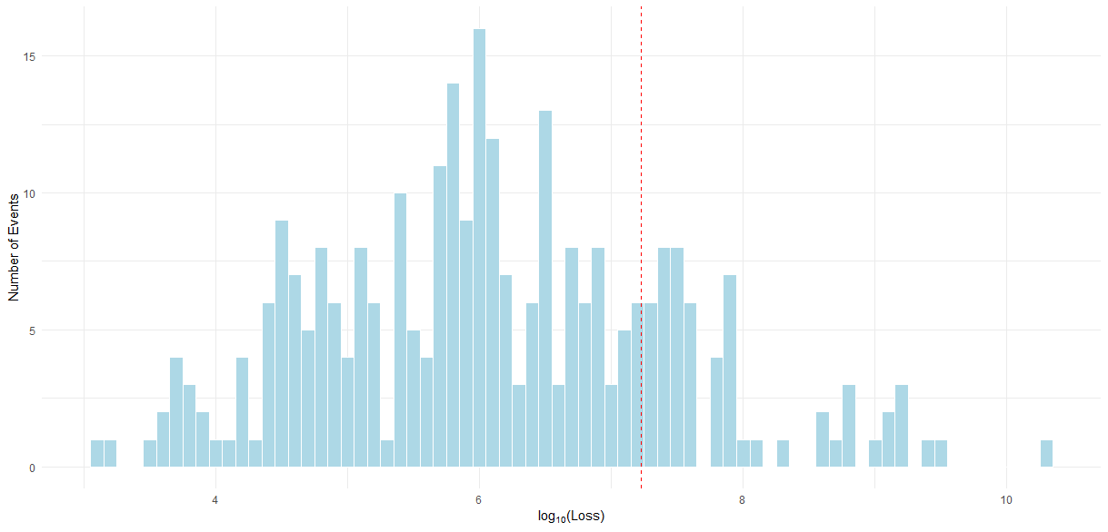
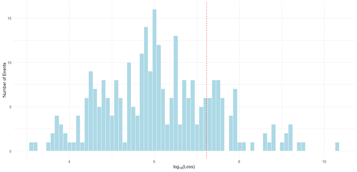
The wildfire data include the date of occurrence, location, and inflation-adjusted (in 2022 US dollars) property loss from direct damage associated with wildfires that occurred in California between 1962 and 2022. Figure 3.1 plots a histogram of the log-transformed losses. The right-skewed distribution suggests the presence of rare but high-severity events.
To prepare the data for modeling, we perform a series of preprocessing steps. First we remove records with zero or missing loss values, then divide all losses by a factor of to improve numerical stability during estimation; therefore, losses are expressed in units of US$100,000.
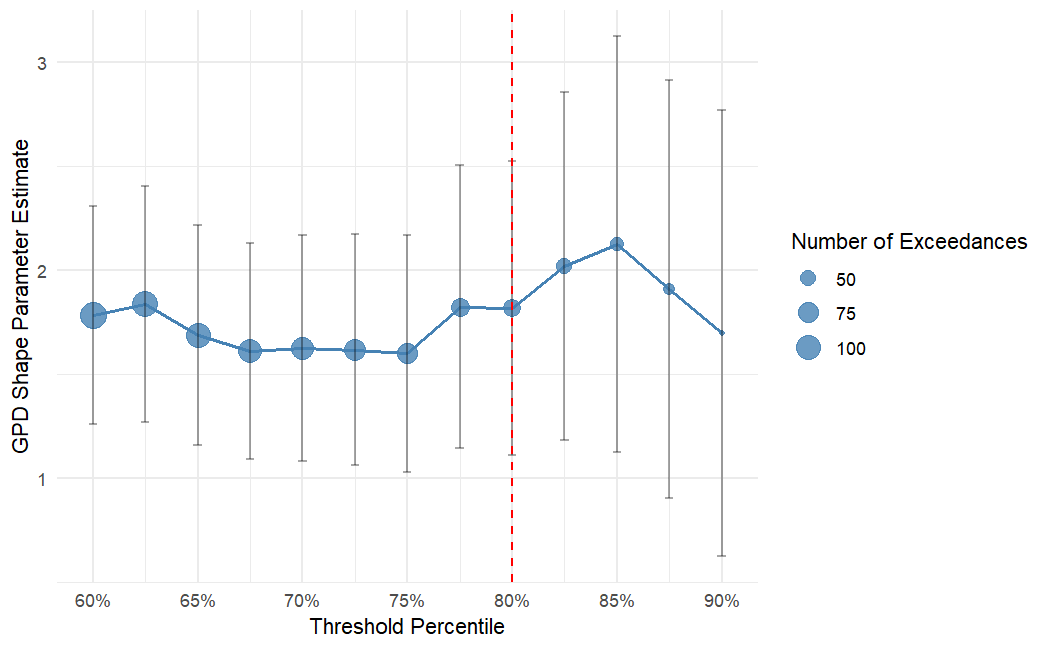
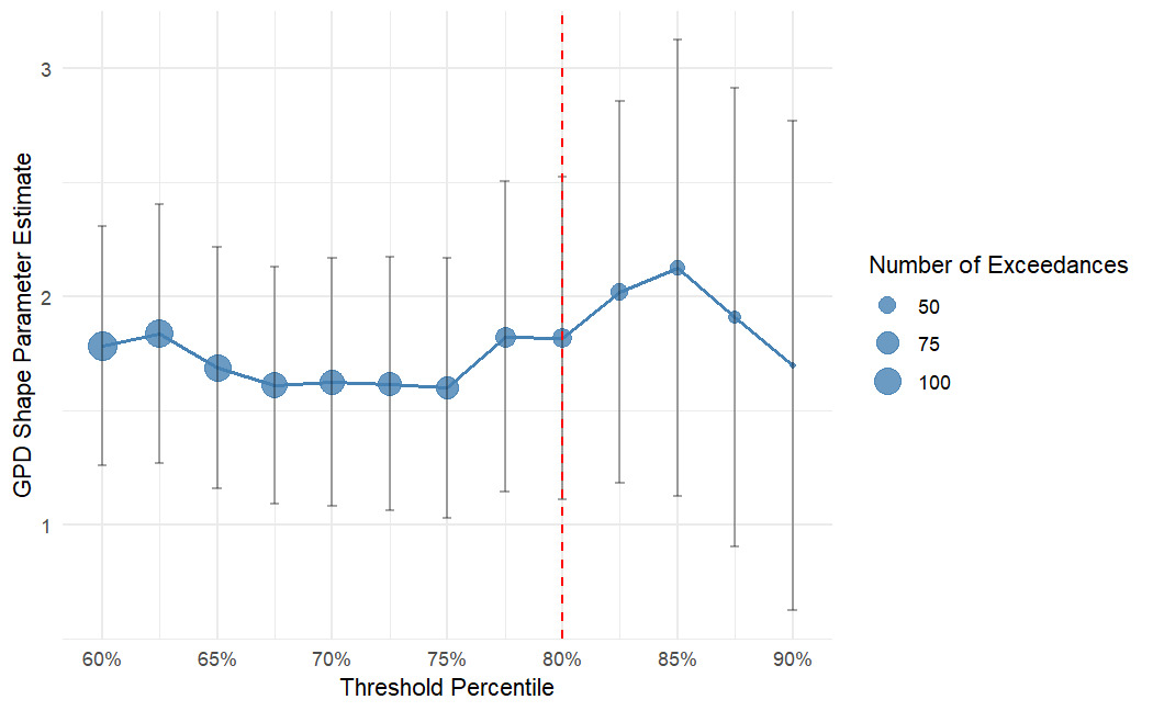
Another important consideration is selecting the threshold used to define exceedance losses, which should be sufficiently high to permit an appropriate GPD approximation and should retain enough exceedances to permit reliable parameter estimation. A commonly used diagnostic is the stability of the estimated GPD shape parameter across a range of candidate thresholds.
Figure 3.2 reports the estimated shape parameter for candidate thresholds corresponding to different percentiles of the losses. At each candidate threshold, we fit a standard GPD to the associated exceedances. The estimates of remain reasonably stable at around the 80th percentile, so this becomes the threshold for defining exceedance losses (indicated by the red dashed line in Figure 3.1). We retain only observations above this threshold and calculate exceedance losses as the amounts by which the observed losses exceed the threshold.
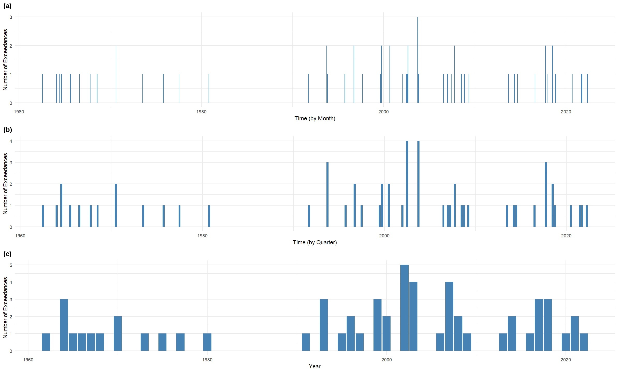
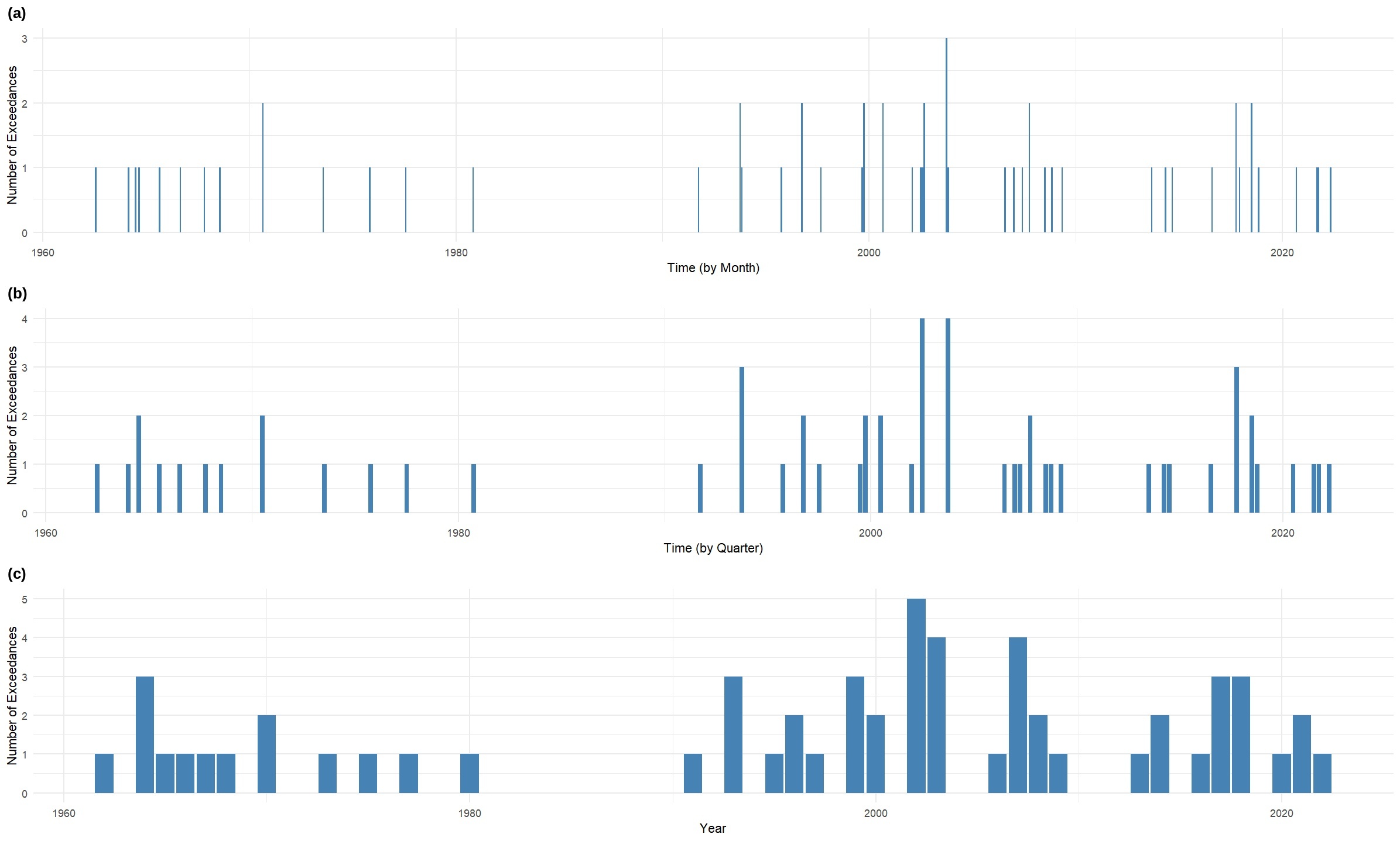
After preprocessing, 58 threshold exceedances remain. Figure 3.3 shows the frequency of these events, grouped by month, quarter, and year. Importantly, these plots clearly show a clustering pattern of extreme wildfire events. Such clustering may arise from seasonal effects, such as elevated wildfire risk during warmer months, or from a self-exciting effect, possibly driven by prior wildfires that further reduce local humidity. The statistical significance of individual clustering sources cannot be identified from visual inspection alone. This motivates a formal statistical inference of seasonal and self-excitation components in modeling extreme wildfire dynamics, as discussed later in Section 3.3.
3.2. Seasonality of wildfires
In the self-exciting POT model, seasonality is captured through the baseline intensity function in equation (2.1). When extreme events exhibit seasonal variation, can be specified as a periodic function to capture predictable fluctuations in event frequency. The specific form adopted for in our case study is described below.
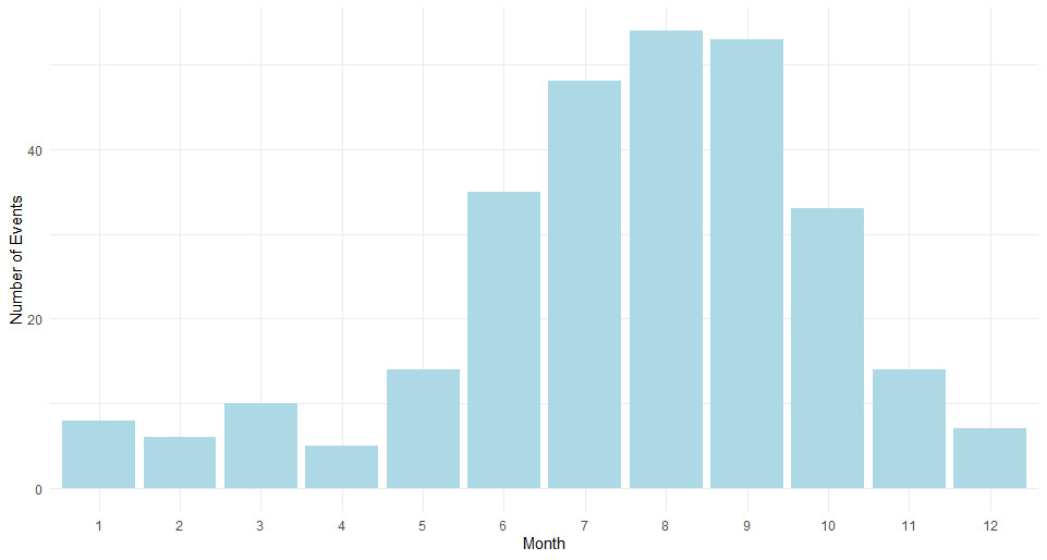
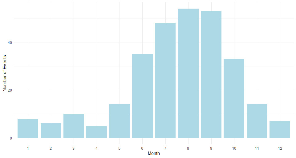
We plot the number of wildfire occurrences grouped by month in Figure 3.4, which shows that occurrences peak between June and October, whereas the remaining months exhibit much lower levels, consistent with the observations of Westerling et al. (2003) and Coogan et al. (2020). This motivates us to distinguish between June through October and the remainder of the year and to specify as a periodic function that is piecewise constant within each year, which is a common practice in point process applications (see, e.g., Bowsher 2007).
Specifically, for any denote by its floor and by its fractional part. We assume that the baseline intensity function is given by
\[ \nu_0(t)=\left\{ \begin{array}{ll} b_2, & \frac{5}{12} < \{t\} \leq \frac{10}{12},\\ b_1, & \text{otherwise}, \end{array} \right. \tag{3.1}\]
where and are nonnegative constants representing the baseline intensity levels during the off-peak and peak wildfire months, respectively. The resulting baseline function provides an approximation to the seasonality pattern of wildfires in the western United States, as illustrated in Figure 3.4 and also in Westerling et al. (2003, Fig. 1).
3.3. Model comparisons
To assess whether seasonality and self-excitation are significant drivers of clustering in extreme wildfire events, we compare models (a)–(d) introduced in Section 2.1. Model (a) serves as the baseline and attributes clustering solely to seasonality. Model (b) introduces a self-excitation component into the intensity process, and model (c) introduces a self-excitation component into the severity distribution. Finally, model (d) represents the full specification that incorporates self-excitation in both the intensity process and the severity distribution.
3.3.1. In-sample goodness-of-fit assessment
We use the maximum likelihood estimation method described in Section 2.2 to calibrate the parameters. The estimation results are presented in Table 3.1. We note that the parameters and in the baseline intensity function in equation (3.1) are statistically significant at the 99% level across all four models. Moreover, the estimates of are significantly larger than those of which indicates a substantial increase in extreme wildfire occurrences during the peak wildfire season from June to October compared with the rest of the year. This confirms the seasonality pattern observed in Figure 3.4 and suggests that seasonality is a significant driver of wildfire clustering during the peak season.
It is also worth noting that the estimated GPD shape parameter in the baseline and baselinefrequency models, both of which exclude a self-excitation component in the severity distribution, is much larger than the corresponding estimates in the models that incorporate severity self-excitation. This suggests that, in the absence of severity self-excitation, the estimate of tail index is forced to absorb unmodeled clustering in large losses. Such large estimates have important implications for short-horizon loss variability and risk concentration, as discussed in Section 3.4.
Another look at the model estimates reveals that the intensity self-excitation term is statistically significant in the full model at the 95% level but not in the baselinefrequency model. This difference arises because the baselinefrequency model restricts clustering to operate only through event arrivals while treating excess loss magnitudes as conditionally independent. In the presence of clustered large losses, this restriction represents a model misspecification. This forces part of the clustering dynamics to be absorbed by the severity distribution, and eventually results in an inflated estimate of yet a weakened identification of the intensity self-excitation effect. Once severity self-excitation is incorporated in the full model, clustering in loss magnitudes is also modeled explicitly; hence, the intensity self-excitation component captures arrival clustering more precisely and emerges as statistically significant.
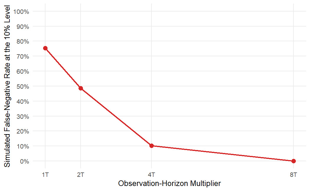
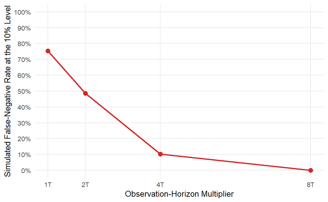
Also of note, the estimated severity self-excitation parameter is not statistically significant. This may reflect the limited information in the current dataset for identifying the severity self-excitation effect. To investigate this possibility, we conduct a simulation study to assess the statistical power of the Hessian-based Wald procedure using observation horizons of and where denotes the actual observation horizon available in the dataset.
Specifically, we simulate data from the fitted full model, with the severity self-excitation parameter set equal to its fitted value. The full model is then reestimated for each simulated dataset, and the significance of the severity effect is evaluated with the same Hessian-based procedure used in our analysis. A false negative is recorded whenever the positive severity effect is not detected at the 10% significance level.
Figure 3.5 shows that the false-negative rate is high at but declines quickly as the observation horizon expands. This result indicates that, even when the data-generating value of is strictly positive and equal to its fitted value, a sample with the same observation horizon as the available dataset often fails to detect the effect as statistically significant.
Next, we further assess the roles of self-excitation in frequency and severity by comparing models (a)–(d) using the log-likelihood, AIC, and BIC criteria. The results are reported in Table 3.2. The baseline model, which incorporates the seasonality component in equation (3.1) but excludes both self-excitation components, exhibits the poorest performance across all evaluation metrics, which indicates its inability to adequately model the dynamics of extreme wildfire losses. Adding the frequency self-excitation component leads to a modest improvement over the baseline model, whereas adding the severity self-excitation component yields a substantial enhancement in model fit. These findings suggest that both self-excitation components contribute to explaining the occurrence and magnitude of wildfire-induced losses. This is further supported in that, despite its slightly greater complexity, the full model achieves the highest log-likelihood and the lowest AIC and BIC values.
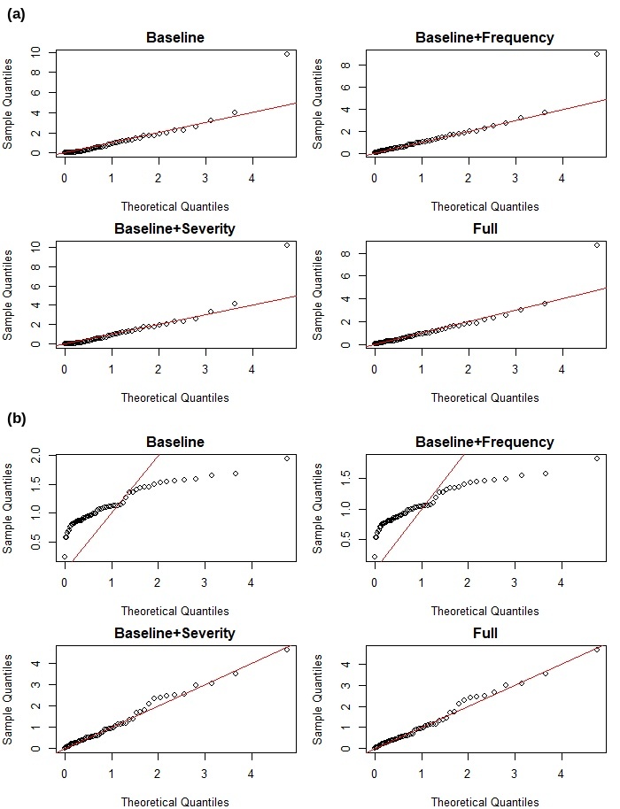
To provide a more comprehensive assessment of goodness of fit, we conduct the KS and AD tests for the two sets of residuals in equations (2.8) and (2.9) for each model. The KS test is sensitive to overall distributional discrepancies, and the AD test places a greater weight on tails. The p-values of these tests are reported in Table 3.3. In addition, Figure 3.6 presents QQ plots of the two sets of residuals against the theoretical quantiles of the standard exponential distribution, which provides a visual evaluation of the distributional fit.
The baseline model again exhibits the poorest performance. It fails both the KS and AD tests for the two sets of residuals, with p-values less than 0.05, and its QQ plot for the residual marks shows clear deviations from the theoretical quantiles. Similarly, the baselinefrequency model does not yield any significant improvement—it fails both tests for the residual marks at the 0.01 level and performs very poorly in the corresponding QQ plot.
In contrast, both the baselineseverity model and the full model exhibit much better alignment in their QQ plots for the residual marks. However, in the KS and AD tests, the baselineseverity model shows a relatively poor fit for the residual inter-exceedance intervals, with low p-values. Conversely, the full model yields high p-values in both tests for the two sets of residuals, which suggests that it provides an adequate fit for both occurrences and extreme losses.
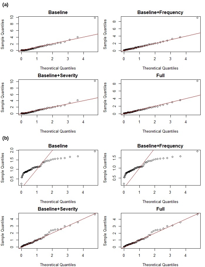
In summary, as shown in Table 3.1, the self-excitation coefficient associated with frequency is statistically significant at the 95% level, indicating that temporal clustering in wildfire occurrences is partly driven by self-excitation. Although the severity self-excitation parameter is not statistically significant at the 90% level, its inclusion substantially improves overall model performance, particularly in the KS and AD tests reported in Table 3.3 and the QQ plot of residual marks shown in Figure 3.6. Taken together, these results support the conclusion that the full model provides the best fit among the four models, and thus, self-excitation in both frequency and severity plays an important role in modeling wildfire losses.
3.3.2. Out-of-sample predictive assessment
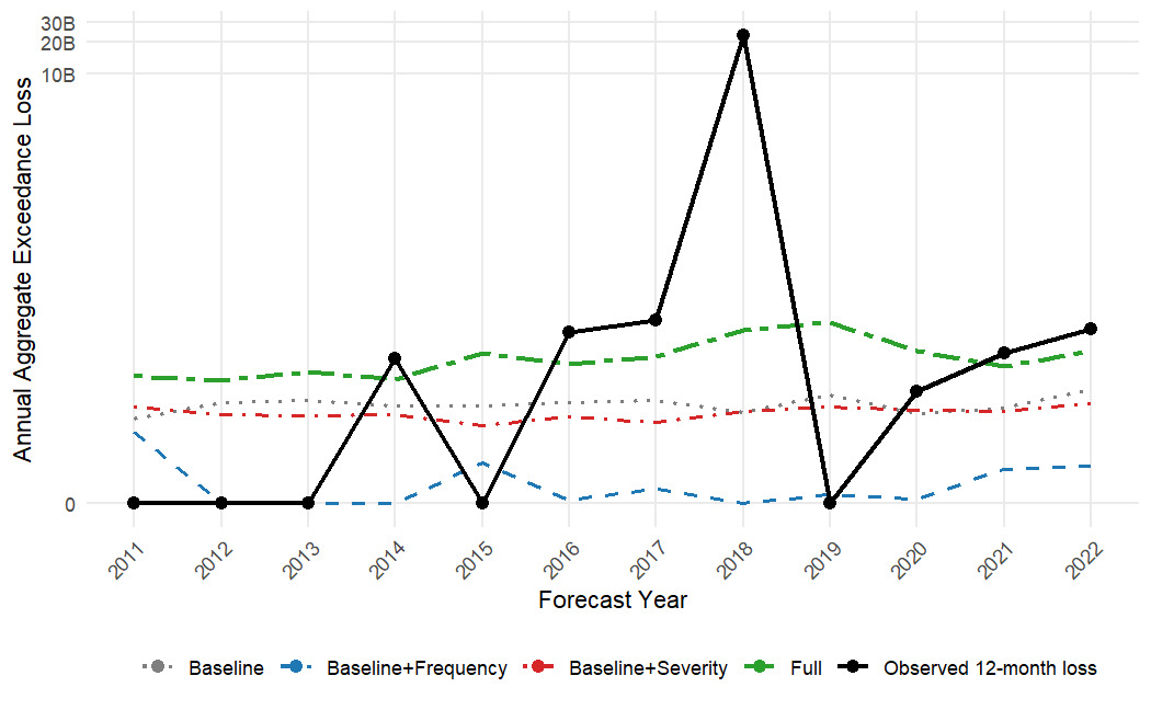
Next, we evaluate the out-of-sample performance of the four models. The comparison provides additional evidence that the full model outperforms the alternatives. We conduct an out-of-sample predictive assessment over the held-out period using model parameters estimated once from the 1962–2010 training sample. At each forecast origin, which advances by 12 months, we use the four fitted models to simulate the aggregate exceedance loss over the following 12 months, conditional on the event history observed up to that time. Thus, the parameter estimates remain fixed throughout the evaluation period, and the conditioning information set expands as newly observed events become available. We then compare the predictive median from each model with the observed annual aggregate exceedance loss. We report predictive medians rather than predictive means because the exceedance severity distribution is heavy tailed. Predictive means can be heavily affected by a small number of extremely large simulated losses and may therefore be unstable as a measure of central predictive performance.
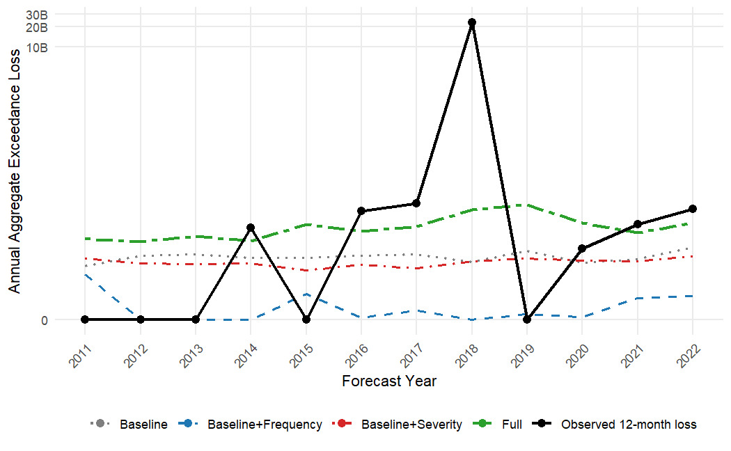
Figure 3.7 shows that, relative to the other three models, the predictive medians from the full model more closely track the observed aggregate losses in years with nonzero but nonextreme losses. This result suggests that jointly modeling frequency and severity self-excitation improves the central predictive performance of the model in typical held-out years. However, extreme realizations remain difficult to predict using only the event history.
Interestingly, the baselinefrequency model often produces zero median forecasts. This pattern arises from how the frequency component is estimated. In the baseline model, the event intensity depends only on the seasonal baseline component. Once frequency self-excitation is introduced, part of the event occurrence risk shifts from the persistent seasonal baseline component to the event-triggered component Consequently, the fitted seasonal baseline in the baselinefrequency model can be lower than that in the baseline model. At many annual forecast origins, the time-decaying effect of previous occurrences is small. Before a new event occurs during the forecast year, the baselinefrequency model may therefore imply a relatively low event intensity.
3.4. Simulated extreme wildfire losses under different models
This section examines how alternative model structures shape the short-term distribution of extreme wildfire losses. The aim is to provide a simulation-based perspective on how self-excitation in frequency and severity affects the aggregate loss distribution over a short time horizon.
To this end, we simulate extreme wildfire losses under the four model specifications described in Table 2.1 using the corresponding parameter estimates reported in Table 3.1 and aggregate them by month. We note that, because model estimation is based solely on losses exceeding the 80th percentile, the simulated severity samples represent excess losses above this threshold. Therefore, each simulated aggregate loss corresponds to the sum of raw losses that exceed the 80th percentile, rather than the total wildfire loss for the corresponding month.
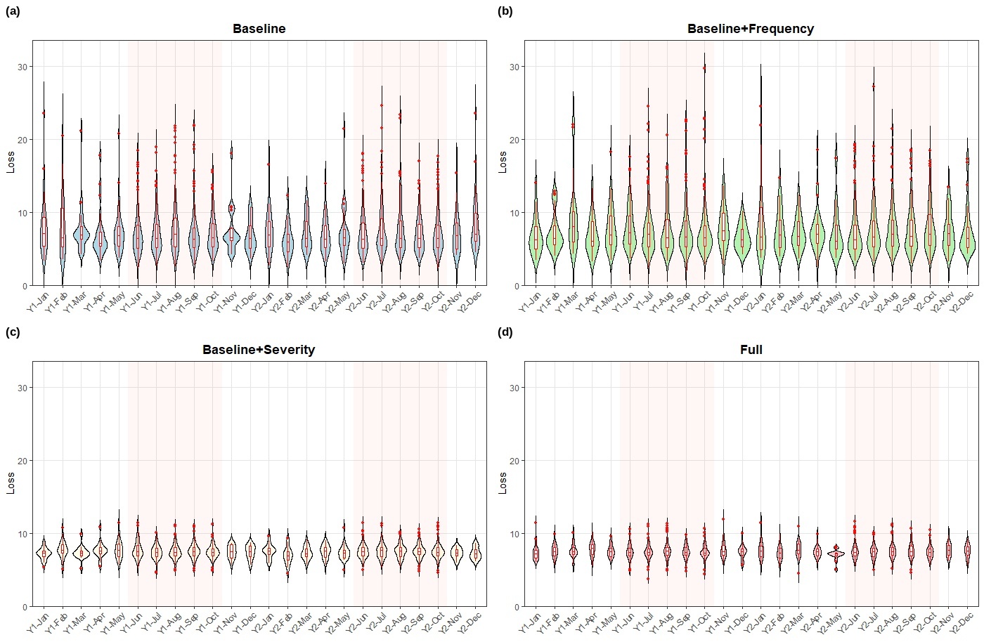
We consider a two-year window since property–casualty insurance contracts are typically short term, and model uncertainty increases as the time horizon widens. We divide the horizon into 24 monthly bins. For all four models, extreme event occurrence times are generated using the thinning method of Lewis and Shedler (1979), which is a standard approach for simulating a nonhomogeneous Poisson process with time-varying intensity. For each event occurrence, a loss value is then sampled from a GPD, with parameters determined by the corresponding model specification. Given the short simulation window, the sparsity of extreme events, the inherent randomness of the GPD, and the path-dependent nature of all models except the baseline, individual sample paths can exhibit substantial variability. We therefore perform 1,000 Monte Carlo replications for each model. To reduce the dominance of the extreme right tail and facilitate meaningful comparison across models, we compute log-transformed aggregate loss values within each month for each run, and then adopt violin plots to visualize the full empirical distribution of simulated losses by month.
As shown in Figure 3.8, the four model specifications produce substantially different patterns for monthly aggregate loss distributions. Compared with the other two models, the baseline and baselinefrequency models exhibit a large number of extreme outliers, with simulated log-loss values frequently exceeding 25 and occasionally approaching 30. This randomness can be directly related to the parameter estimates in Table 3.1. In particular, the estimated GPD shape parameters for these two models are as large as and respectively. Such large values imply extremely heavy-tailed severity distributions, under which extreme losses occur with disproportionately high probability. These extreme losses can then propagate through the self-excitation mechanism, amplifying subsequent loss occurrences and severities, and eventually resulting in aggregate loss distributions with excessive variability. This provides additional evidence that self-excitation should be incorporated to capture the distributional characteristics of extreme wildfire losses.
In contrast, the baselineseverity and full models produce tighter predictive distributions. The number and magnitude of outliers are greatly reduced. This improvement demonstrates the role of severity self-excitation in adapting the scale of the loss distribution to recent event history, which in turn mitigates the tendency to generate unrealistically extreme losses. Although the difference between the simulated aggregate loss distributions of the baselineseverity and full models in Figure 3.8 is not apparent, this aligns with the results in Section 3.3, which suggest that severity self-excitation operates on a relatively moderate yet non-negligible scale.
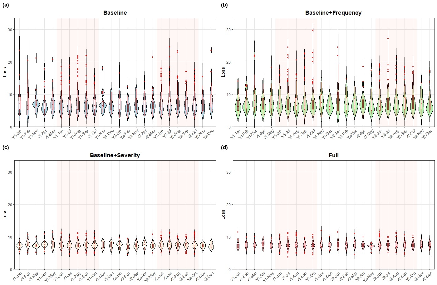
The simulation findings in Figure 3.8, together with the comparison of model evaluation metrics and residual tests for the two sets of residuals across all four models in Section 3.3, suggest that incorporating self-excitation in both frequency and severity is important for producing a stable and realistic short-horizon predictive distribution of extreme losses.
4. Concluding remarks
We use a self-exciting POT model to jointly model the frequency and severity of climate-related extreme events, which simultaneously captures the temporal clustering of climate extremes, the time-varying nature of occurrence rates and severity distributions, and the dependence between frequency and severity. Two factors, seasonality and self-excitation, drive the clustering embedded in the model. We illustrate the framework using a case study of California wildfire losses. Our empirical results show that incorporating self-excitation in both frequency and severity improves overall model fit, and that the self-excitation component in frequency is statistically significant at the 95% level. Although the severity self-excitation component is not statistically significant (possibly because of the limited statistical power of the Hessian-based significance test), incorporating this component substantially improves the overall model fit, increases the accuracy of median predictions, and enhances the model’s ability to capture short-horizon variability in extreme wildfire losses. Together, these findings highlight the importance of modeling self-excitation in both frequency and severity alongside seasonality when assessing climate-related extreme risks.
Our empirical study demonstrates that the self-exciting POT model provides superior in-sample fit. Future research could extend the model by incorporating exogenous climate covariates, such as drought indices or large-scale climate oscillations, into both the frequency and severity components. In addition, because our analysis focuses on a single peril and geographic region, it would be valuable to examine whether the findings generalize to other climate hazards and locations.
See the list of companies in the Receivership process at https://www.myfloridacfo.com/division/receiver/companies (Accessed: October 1, 2026).